A Beginner’s Guide to Continual Learning

I am currently researching on continual learning, a paradigm of machine learning. I am keen to introduce its basic knowledge here to who are interested in this field or just in what I’m doing personally. I’m going to explain the basics of continual learning including concepts, problem definition, datasets, metrics, etc, and go through some selected classic algorithms in each of the method categories (without too many details). I also attached a list of other continual learning resources made by me in the end if you want to learn more.

Slides for this post: Learning with Non-Stationary Streaming Data: A Beginner’s Guide to Continual Learning

1 Continual Learning and Related Concepts

Continual learning is also known as lifelong learning, incremental learning and sequential learning. Just a bit of history, this field started in 1990s when it was usually referred to as lifelong learning, but now continual learning is more common after deep learning was brought to this field and made it thrive again.

1.1 The Scope

First things first, it’s very important to understand the scope of this concept: continual learning is one of the machine learning paradigms. So what are machine learning paradigms?

We often come across a variety of different terms when looking up machine learning, such as supervised / unsupervised learning, reinforcement learning, transfer learning, or perhaps image classification, object detection, machine translation if you are into real applications more. There are many mixed usages among the words like scenarios, tasks, settings, problems, but here I make clear definitions for these terms. We call the real applications as scenarios, and the more abstract concepts as paradigms. Formally, paradigms are concerned with how data are distributed, the way that they are allowed to be used, and how the model is evaluated, without considering the types of data themselves.

Supervised and unsupervised learning are probably the most commonly seen paradigms. They are concerned with general components of the data – whether labels are used for training, and typically involve one-off training and testing process (which we often refer to as a task). Over the past decade, many problems involving multiple tasks caught attention of machine learning researchers and evolved into paradigms which led to increasing popularity of keywords in deep learning research. These include, but are not limited to: transfer learning, multi-task learning, online learning, meta learning, and of course, continual learning.

1.2 Definition

At the conceptual level, I define continual learning as follows:

Definition 1 (Continual Learning) A multi-task machine learning paradigm where an algorithm receives the data from tasks sequentially without the access to previous ones to learn a model that performs the best for all tasks.

It’s important to note that “sequentially” and “for all tasks” are both essential to this concept. Continual learning could turn to other paradigms without either of them. See Section 1.3 for details.

The non-accessibility to previous task is also a key distinction of continual learning. It is a very practical assumption, considering the substantial memory costs or potential privacy concerns associated with storing all previous data in real-world scenarios.

If access to data from previous tasks is allowed, the model can actually be retrained using all data from both the new and previous tasks, which is sometimes called joint training. However, it is not even better. Aside from the increasing computational cost, the data from various distributions make learning difficult as well. The model might either learn overly general patterns that fail to benefit all tasks, or it could learn incorrect patterns (a problem sometimes referred to as induction bias). Multi-task learning paradigm attempts to address this challenge, but in continual learning it is not worth the overhead of training a multi-task model multiple times.

It’s also important to note that continual learning involves an infinite sequence of tasks, so the algorithm has no idea about future challenges. This is what “continual” is meant for.

Additionally, continual learning typically deals with tasks that are significantly different from one another. If the tasks were from the same distribution or were highly similar, it wouldn’t be a challenge for the algorithm to perform well across all of them. In other words, the data stream is usually non-stationary (assuming we blur the boundaries between tasks).

As this is the definition chapter, I would like to introduce more specific concepts such as TIL and CIL, but they cannot be explained in an abstract way for now. I’ll come to that later after the definition of continual classification problem in Section 2.1 and Section 2.2.

1.3 Differences From Other Paradigms

The differences from other paradigms, as we said, depend on how the data used (training) and evaluated (testing) are organised. Figure 1 shows clearly the differences on data usage between paradigms concerning multiple tasks.

Figure 1: Illustration about differences among Multi-task paradigms. (Source: De Lange et al. 2021)

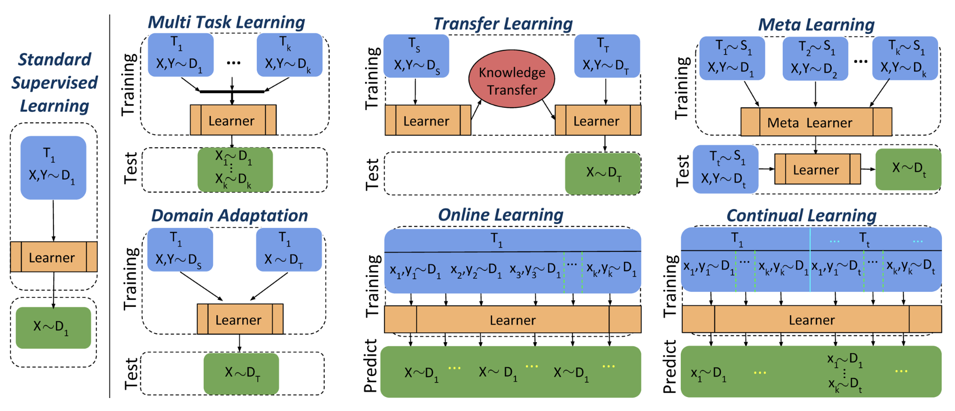
• Standard supervised learning: continual learning with one task reduces to this conventional machine learning paradigm.
• Multi-task learning: if continual learning does not involve “sequentially,” the algorithm has access to data from each task all at once when training on the final task, which becomes multi-task learning.
• Transfer learning / domain adaptation: if continual learning does not involve “for all tasks,” the algorithm’s goal becomes the performance on the final task alone, which becomes similar to transfer learning. If it focuses on tasks other than the final one, it resembles a less common paradigm known as reverse transfer learning. Note that transfer learning usually involves just two tasks (A & B). Domain adaptation is closely related to transfer learning.
• Online learning: this is essentially a single-task paradigm where testing and application occur as frequently as the training data. While it may seem similar to continual learning, the key difference is that in online learning, all data comes from the same distribution.
• Meta learning: if “for all tasks” in the definition of continual learning is replaced with “for unseen new tasks,” it becomes meta learning. In this case, the algorithm lacks any supervisory information for unseen tasks, so it must learn how to learn. This process is handled by a meta-learner that treats tasks as samples for learning at a higher, meta level.

1.4 Why Continual?

There are many aspects to human learning. One of the most important is the ability to learn and adapt new knowledge continuously without forgetting previous knowledge. Unfortunately, this is difficult to achieve through standard deep learning processes. Therefore, a wide range of paradigms, as mentioned earlier, have been explored from different perspectives to equip AI not only with strong performance on a single task but also with the ability to handle multiple tasks. Continual learning is the paradigm primarily focused on addressing the problem of forgetting in neural networks (this problem is commonly referred to as catastrophic forgetting, which we will discuss later).

Continual learning is still in its early age without so many examples of applications due to its difficulty, but it is a highly promising solution for real-world applications facing continuous streams of non-stationary data, where retraining from scratch is impractical. Here are some examples:

• In Robotics
  • Robotic agents are naturally playground for continual learning because they interact with the real world. Some even says CL is born for robotics. There are various scenarios like object detection, segmentation, reinforcement learning often face the non-stationary data challenges (Lesort et al. 2020).
• In Autonomous Driving
  • The environment and driving conditions are constantly changing, like weather, traffic and objects (Verwimp et al. 2023; Shaheen et al. 2022).
• In Finance
  • For example, anomaly detection in auditing (Hemati, Schreyer, and Borth 2021): a company might face different patterns of frauds in their financial quarters or years. Other applications could be like algorithm trading, portfolio selection (Liu et al. 2023), financial forecasting (Singh et al. 2023), credit scoring.
• Other areas of applications: CV, NLP, recommendation systems, health care, etc, can also be fitted in continual learning.

2 Continual Classification Problem

In the field of continual learning, most researchers limit their scenarios to classification tasks, especially image classification. This is not only because classification is the most basic scenario in machine learning, but also because of the difficulty of continual learning itself. Perhaps people don’t want to make things more complicated before improving performance on simple applications. Here we provide a formal definition of classification problem in continual learning.

Definition 2 (Continual Classification Problem)  

• Tasks: $t=1,2,\cdots$
• Training data of tasks: ${\mathcal{D}}_{\text{train}}^{(t)}=\{({\mathbf{x}}_i,y_i){\}}_{i=1}^{N_t}\in ({\mathcal{X}}^{(t)},{\mathcal{Y}}^{(t)})$
• Testing data of tasks as well: ${\mathcal{D}}_{\text{test}}^{(t)}\in ({\mathcal{X}}^{(t)},{\mathcal{Y}}^{(t)})$

We aim to develop an algorithm that trains the model $f^{(t-1)}$ to $f^{(t)}$ at the time for task $t$:

• With access to ${\mathcal{D}}_{\text{train}}^{(t)}$ only.
• To perform well on all seen tasks ${\mathcal{D}}_{\text{test}}^{(1)},\cdots ,{\mathcal{D}}_{\text{test}}^{(t)}$

Again, the distributions $({\mathcal{X}}^{(t)},{\mathcal{Y}}^{(t)}),t=1,2,\cdots$ are usually very different from each other. They can be totally different tasks, from classifying handwritten numbers to classifying animals, or from binary to multi-class classification.

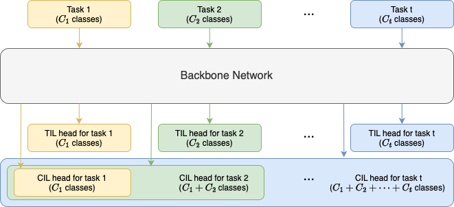
You might wonder at this point, how can a model $f$ with the same architecture deal with different tasks? At least, a model for binary classification certainly cannot handle more than 2 classes in a new task. The answer is, a neural network architecture for continual learning is always a multi-head classifier where the output heads are assigned to the tasks. A head is simply a linear output layer for a shared $f$ to the maximum extent. New heads are initialised and trained along with $f$ as new tasks come in.

In terms of the way to test different tasks, continual learning classification can be divided into subcategories of TIL and CIL. They have different logics in their output heads:

Figure 2: Difference between the output heads of TIL and CIL continual learning.

We introduce TIL and CIL as follows. Let’s assume that task $t$ contains $C_t$ classes.

2.1 Task-Incremental Learning (TIL)

Task-Incremental Learning (TIL) provides the model with information about which task an instance belongs to during testing. In other words, the test instance is $(\mathbf{x},y,t)$, where $(\mathbf{x},y)\in ({\mathcal{X}}^{(t)},{\mathcal{Y}}^{(t)})$. This is similar to how A-level exams are conducted separately for each subject, with students knowing exactly which subject they are being tested on.

In this case, the output heads for different tasks can be completely segregated. As shown in Figure 2, a TIL head is created solely for its new task because it doesn’t have to consider other tasks.

Note

If the task ID information is not provided for test instances, it becomes a more challenging paradigm, which I call task-agnostic testing (though it is less commonly used). In this case, the model must figure out the task ID by itself.

There are even more advanced paradigms that eliminate the task boundary. For example, task-agnostic continual learning assumes that task IDs are not even given during training. We will not cover these paradigms here.

2.2 Class-Incremental Learning (CIL)

Class-Incremental Learning (CIL) mixes classes from all tasks together and let the model choose from a class that could be from any seen task. That is, the test instance is $(\mathbf{x},y)\in ({\mathcal{X}}^{(1)}\cup \cdots \cup {\mathcal{X}}^{(t)},{\mathcal{Y}}^{(1)}\cup \cdots \cup {\mathcal{Y}}^{(t)})$. You can imagine a huge session of A-level exam that includes and mixes all the subjects in one single paper. CIL drops the assumption that the model knows the task ID, making it much more difficult than TIL, especially as the task sequence goes longer.

In CIL, the output heads therefore evolve incrementally, as shown in Figure 2. The model uses the large final output head, which inherits all the previous heads, to perform testing, rather than to identify the independent head of a known task ID.

3 Challenges: Insights from Baseline Algorithms

Continual learning is currently a very difficult learning paradigm due to challenges like catastrophic forgetting and the trade-off between model stability and plasticity. In this chapter, I will show the effects of 2 baseline algorithms, which push the model to either extreme of stability or plasticity. Hopefully, these examples will make the challenges I’m going to talk about later more intuitive.

Before getting into the baseline algorithms, let’s look at some preliminaries: where the challenges are evaluated (datasets) and how they are quantified (metrics).

3.1 Datasets: Permute, Split, Combine

The datasets used to evaluate continual learning algorithms are typically sequences of standard machine learning datasets. These datasets are usually constructed in three ways:

1. Combine: datasets from different sources are used, each serving as a separate task. For example, HAT is evaluated on a sequence consisting of 8 datasets: CIFAR10 and CIFAR100, FaceScrub, FashionMNIST, NotMNIST, MNIST, SVHN, and TrafficSigns. (Note that these datasets may have different input dimensions, so it’s necessary to either align the inputs or design task-specific model inputs accordingly.)
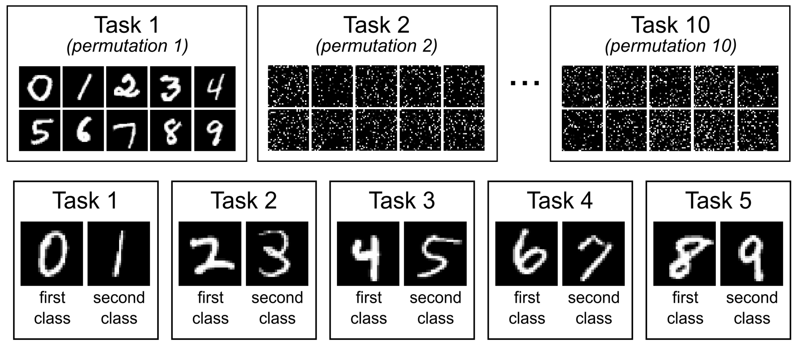
2. Permute: in this case, a single dataset is modified by permuting the images in some way to create different tasks. The top half of Figure 3 shows the Permuted MNIST dataset. Note that permutations must be applied in a consistent manner to create a valid dataset. That’s why permutation seeds are set, to avoid completely randomising the dataset which makes nothing is able to be learned.
3. Split: A dataset usually contains multiple classes, and these classes can be grouped together to form smaller datasets. The bottom half of Figure 3 shows the Split MNIST dataset, spliting MNIST into 5 tasks, each of which has 2 classes. This is another approach to creating tasks.

Figure 3: Permuted and split MNIST datasets. (Source: Van de Ven and Tolias 2019)

Permute and split are the ways to construct a sequence of tasks from one single dataset. They are more commonly used in continual learning research. All the methods can be used to construct any of TIL, TIL with task-agnostic testing, CIL.

3.2 Metrics: What CL Cares About

Although the task sequence in CL may be infinite, we have to stop at some point to take a look at how well the model is performing. In papers and benchmarks, the number of tasks is typically for evaluation purposes, allowing for comparison between CL algorithms under a consistent standard.

The evaluation after training on task $t$ involves testing all previously seen tasks, $\tau =1,\dots ,t$. For each task $\tau$, the test is conducted on ${\mathcal{D}}_{\text{test}}^{(\tau )}$, and the model’s performance (e.g., classification accuracy) is recorded. Using accuracy as an example, we denote the performance on task after training task $t$ as $a_{\tau ,t}$, which forms an lower triangular matrix of metrics. This matrix plays a key role in evaluating continual learning, and all other metrics are derived from it (along with a few additional auxiliary measures).

$$\begin{array}{cccc}{a}_{1,1}& & & \cdots \\ a_{2,1}& a_{2,2}& & \cdots \\ a_{3,1}& a_{3,2}& a_{3,3}& \cdots \\ ⋮& ⋮& ⋮& \ddots \end{array}$$

As previously mentioned in the definition, the primary goal of continual learning is to ensure that the model performs well on all tasks. Therefore, the average accuracy (AA) serves as the key performance metric, reflecting this overall objective. All efforts in continual learning aim to improve this metric.

$${\mathrm{AA}}_t=\frac{1}{t}\sum _{\tau =1}^t{a}_{t,\tau }$$

Forgetting is a major challenge in continual learning algorithms. It appears as a decline in performance on previously learned tasks. To quantify this, we have the backward transfer (BWT) metric, which measures the difference in performance between the current accuracy and the accuracy drop on previous tasks (summed up across all combinations of current and previous task pairs). It also reflects the stability of the continual learning model, as a smaller performance drop on previous tasks indicates that the model is kept stable from significantly changed by new tasks.

$${\mathrm{BWT}}_t=\frac{1}{t-1}\sum _{\tau =1}^{t-1}(a_{t,\tau }-a_{\tau ,\tau })$$

Continual learning algorithms definitely have some influence on the training of current task because interaction with previous tasks is involved. They could have achieved better performance without considering preventing forgetting on previous tasks. We call model trained by the task alone the reference model. To quantify how much the current task training is influenced by considering previous tasks, we have the forward transfer (FWT) metric, which measures the difference in performance between continual learning model and the reference model. It also reflects the plasticity of the continual learning model, as the compared reference model is theoretically most plausible model.

$${\mathrm{FWT}}_t=\frac{1}{t-1}\sum _{\tau =2}^t(a_{\tau ,\tau }-a_{\tau }^I)$$

AA, BWT, FWT are the most common metrics in continual learning. They are single values calculated from the matrix reflecting overall properties till learning task $t$, therefore I’d like to call them overall metrics. For a deeper dive into all metrics used in continual learning, refer to another post by me “A Summary of Continual Learning Metrics”.

3.3 Baselines: Finetuning and Fix

This section introduces the two baseline continual learning algorithms, and presents their results on the Permuted MNIST dataset. This provides intuitive insights into the challenges faced by continual learning algorithms.

The most naive way to complete a continual learning process is to take no action and let the model learn from the sequential data of tasks. Specifically speaking, at the beginning of each task, it simply initialises the training as the model learned at the end of the last task. This approach is generally referred to the Finetuning baseline (in some papers, SGD, i.e. Stochastic Gradient Descent). It is technically not a proper continual learning algorithm but early CL work usually took it as a baseline. Note that new output heads are sequentially introduced and Finetuning simply initialises them in the way it was supposed to be.

In experiments with the Permuted MNIST task (10 tasks), as shown in Figure 4, we observe that the model’s performance on the last task drops significantly each time a new task arrives, and continues to drop as more tasks arrive. This leads to a substantial decrease in the average accuracy (AA).

Figure 4: The lower triangular accuracy matrix and overall accuracy of two baseline algorithms, evaluted on Permuted MNIST, 10 tasks.

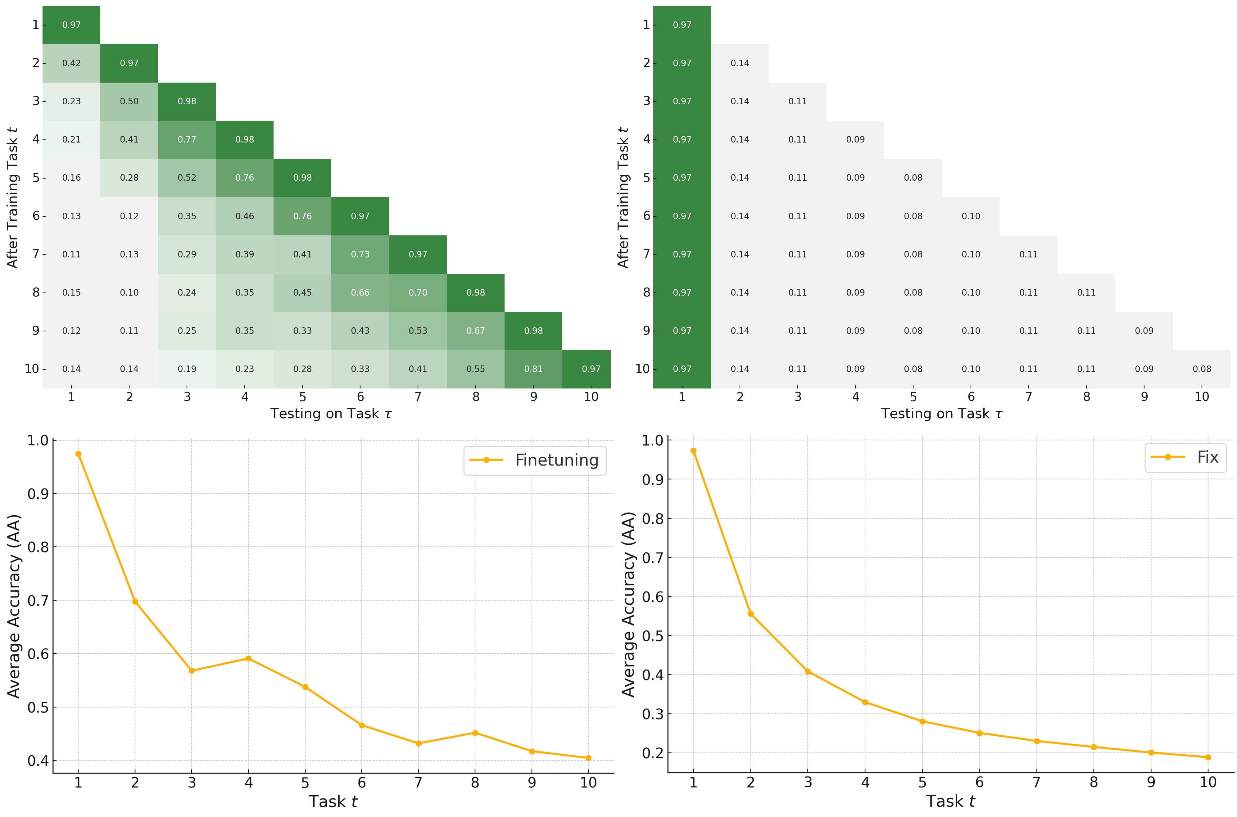
The situation is even worse in CIL setting, where accuracy for tasks except current task can drop to zero due to the absence of negative examples, which highlights that CIL is inherently more challenging than Task Incremental Learning (TIL). This happens because the model is convinced to predict classes from the new task only if it does not know anything about previous tasks. If you know about machine learning, negative examples are very important to machine learning, where many works try to deal with unbalanced data.

We can infer that, the direct cause of the poor performance is that the training on top of previous task is completely unconstrained, causing a lot of forgetting. We can reverse the Finetuning approach, which is the Fix approach. This approach simply fixes the model after the training the first task and stops learning, just aiming to fully address the forgetting problem.

However, this lead the results to the other extreme. On the same experiment settings, Figure 4 shows the performance of new task is way much worse than the first task, which also leads to drop on AA as more tasks come to be calculated into average.

3.4 Challenge 1: Catastrophic Forgetting

Due to the inherent characteristics of neural networks, previous knowledge can hardly be preserved when model converges to data containing new knowledge. This phenomenon reflects a lot in continual learning, where learning new tasks can interfere with and degrade performance on previously learned tasks. It is referred to catastrophic forgetting in deep learning research literature, and considered as the main challenge of continual learning. As we have seen, Finetuning, the naive continual learning algorithm, suffers the most from this problem, and so do many other continual learning algorithms that are modified from the Finetuning framework.

Researchers in continual learning used to focus very much on catastrophic forgetting. Many algorithms are designed to prevent it, once making continual learning equivalent to addressing forgetting. However, it is more regarded in recent years as one side of a broader challenge – stability-plasticity dilemma.

3.5 Challenge 2: Stability-Plasticity Dilemma

Catastrophic forgetting actually reflects low stability of the continual learning model. While Finetuning suffers the low stability problem, we have also seen that, the other extreme, Fix, promotes too much stability and completely lost plasticity. As shown in the baseline results, both of them are very problematic, leading to the drastic drop in performance.

The two baselines show that continual learning models are hard to achieve both high stability and plasticity. Higher stability / plasticity often leads to lower plasticity / stability, like a balance. This indicates that catastrophic forgetting is only one side of a stability and plasticity balance. This is called Stability-Plasticity Dilemma in deep learning, particular explicit in continual learning.

Figure 5: An illustration in the parameter space showing how different continual learning algorithms balance their efforts on current and previous tasks. The ellipses denote the loss contour of the corresponding tasks.

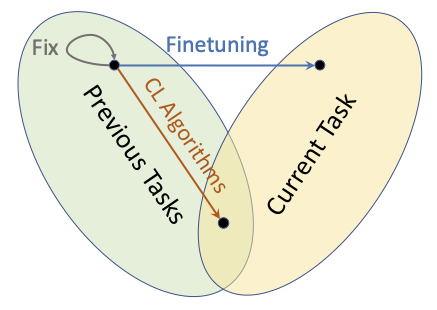
Therefore, a good continual learning algorithm (shown in Figure 5) must strike a balance between the two extremes, aiming to find an optimal point that balances the stability and plasticity of the model. This balance is key to achieving the best average performance. Continual learning is not just about mitigating forgetting; it’s about effectively managing the trade-off between stability and plasticity.

As for the reason why balancing the trade-off leads to better average performance, we could think in another interesting way. If we look at the 2 baselines, we could find they both pour all the effort to achieve the better performance of only one task. Finetuning favourites the last task while Fix prioritises the first task. However, considering the long task sequence in continual learning, it is very unwise to give up all other tasks as the objective takes every task into account.

3.6 Challenge 3: Network Capacity

Learning AI models is also a process of resource allocation. In neural networks, knowledge derived from data is distributed across the model and consolidated into its representation space. In conventional machine learning with single task, the network size is typically chosen based on the data size to avoid underfitting or overfitting. However, when applied to continual learning, this approach encounters a challenge. Knowledge continues to arrive task after task without end assuming an infinite sequence of tasks, making it impossible to pre-select an appropriately sized network since the data size is never known. Any fixed model will eventually reach its capacity, causing performance to degrade. This is the challenge of network capacity.

Some continual learning algorithms adhere to the assumption of a fixed network, but others do not. These algorithms typically expand the network by introducing new parameters—either in a linear or dynamic, adaptive manner—whenever a new task arises or the network reaches its capacity limit.

It is unfair to compare algorithms that assume a fixed network with those that allow for expansion. Imagine that in TIL, a naive algorithm where each new task initialises a completely independent model (which is called independent learning) could easily achieve optimal performance, similar to the reference model mentioned above. (This algorithm is often used as the theoretical upper bound of accuracy in many studies. ) This is why some research advocates for new performance metrics that account for model memory, to ensure a more fair and comprehensive evaluation.

4 Methodology Overview

Since 2017, continual learning has gained significant attention in deep learning research, with various algorithms being proposed. The core idea behind tackling the continual learning paradigm is to retain as much valuable information and knowledge from previous tasks and effectively incorporate it into subsequent ones. Different categories of approaches do this from various aspects of a machine learning system (with one notable exception: architecture-based approaches).

In the following sections, we will explore the most classic continual learning algorithms across these categories, providing a clearer understanding of how continual learning works. Pay attention to how information from previous tasks is utilized and integrated into the learning process, and how architecture-based approaches try to do continual learning in a different way.

4.1 Replay-based Approaches

As mentioned earlier, one of the most vanilla ways to do continual learning is to retrain the model on the new task with all the previous data (joint training), but it violates the assumption of continual learning that no access to previous data. However, it is still allowed to leverage a small amount of previous data, as the assumption is mainly about data memory issue. This is the idea behind replay-based approaches, which select representative data from previous tasks for replaying during future task training. These approaches prevent forgetting by storing parts of the data from previous tasks and using them to consolidate previous knowledge. They are designed to mimic the previous task distribution without accessing the entire dataset.

In fact, the amount of replay data is not sufficient for re-training. It needs to be representative and must be handled differently from simply mixing it into the training batch with data from new task.

One of the earliest replay-based work is iCaRL (Rebuffi et al. 2017). It selects representative samples by some manual filter rules, and uses them as a reference of knowledge distillation for training new tasks. In this work, the memory for replay data is fixed and evenly allocated for each previous task.

4.2 Regularisation-based Approaches

Regularisation-based approaches add regularisation to loss function. The regularisation is a term added to loss function, which is meant for preventing forgetting:

$$\underset{\theta }{min}{\mathcal{L}}^{(t)}(\theta )={\mathcal{L}}_{\text{cls}}^{(t)}(\theta )+\lambda R(\theta )$$

$\lambda$ is the regularisation parameter which works as a hyperparameter controlling the intensity of preventing forgetting, or the scale to balance stability-plasticity trade-off. The more $\lambda$ is, the more the model is constrained to prevent forgetting, which leads to more stability.

The regularisation term is also a function of parameters $\theta$, like the classification loss for the new task: ${\mathcal{L}}_{\text{cls}}^{(t)}(\theta )=\sum _{(\mathbf{x},y)\in {\mathcal{D}}_{\text{train}}^{(t)}}l(f(\mathbf{x};\theta ),y)$.

In various ways of regularisation, some directly regularise on the values of parameters, we call parameter regularisation. The most naive way is to encourage the parameters for the new task close to the parameters trained on previous tasks (which is sometimes called the L2 regularisation):

$$R(\theta )=\sum _i{({\theta }_i-{\theta }_i^{(t-1)})}^2={\Vert \theta -{\theta }^{(t-1)}\Vert }^2$$

Treating all parameters equally is too simple. Some approaches differentiate the parameters by assigning them importance values, thereby applying regularisation in a more nuanced way:

$$R(\theta )=\sum _i{\omega }_i{({\theta }_i-{\theta }_i^{(t-1)})}^2$$

For example, EWC (Elastic Weight Consolidation) (Kirkpatrick et al. 2017) uses the following measure as importance for each parameter, which is calculated after training task $t-1$ and before training task $t$:

$${\omega }_i=F_i=\frac{1}{N_{t-1}}\sum _{(\mathbf{x},y)\in {\mathcal{D}}_{\text{train}}^{(t-1)}}{\left[\frac{\partial l(f^{(t-1)}(\mathbf{x},\theta ),y)}{\partial {\theta }_i}\right]}^2$$

EWC is probably the most widely used and successful approach in continual learning. The formula is derived from a series of statistical inductions, which I won’t delve into here. I just explain intuitively here. For parameter ${\theta }_i$, it represents the gradient of the classification loss with respect to this parameter within the model after training on task $t-1$. This gradient indicates the sensitivity of this parameter to the model’s performance. If the parameter is highly sensitive, it suggests that it plays an important role. The gradient is averaged over the training data, which is assumed to represent the data distribution of task $t-1$.

Some other approaches regularise the parameters indirectly, focusing instead on other components that are functions of the parameters. One example is on features, which is called feature regularisation. The most naive way is to encourage the features extracted by the new model to be similar to those extracted by the previous model. This is actually knowledge distillation from previous tasks into new task, which is the core idea behind LwF (Learning without Forgetting) (Li and Hoiem 2017):

$$R_{\text{LwF}}(\theta )=\sum _{(\mathbf{x},y)\in {\mathcal{D}}_{\text{train}}^{(t)}}l(f(\mathbf{x};\theta ),f(\mathbf{x};{\theta }^{(t-1)}))$$

While this approach is not very effective or sophisticated, it is simple and works reasonably well, which is why it became quite popular in early continual learning studies.

4.3 Architecture-based Approaches

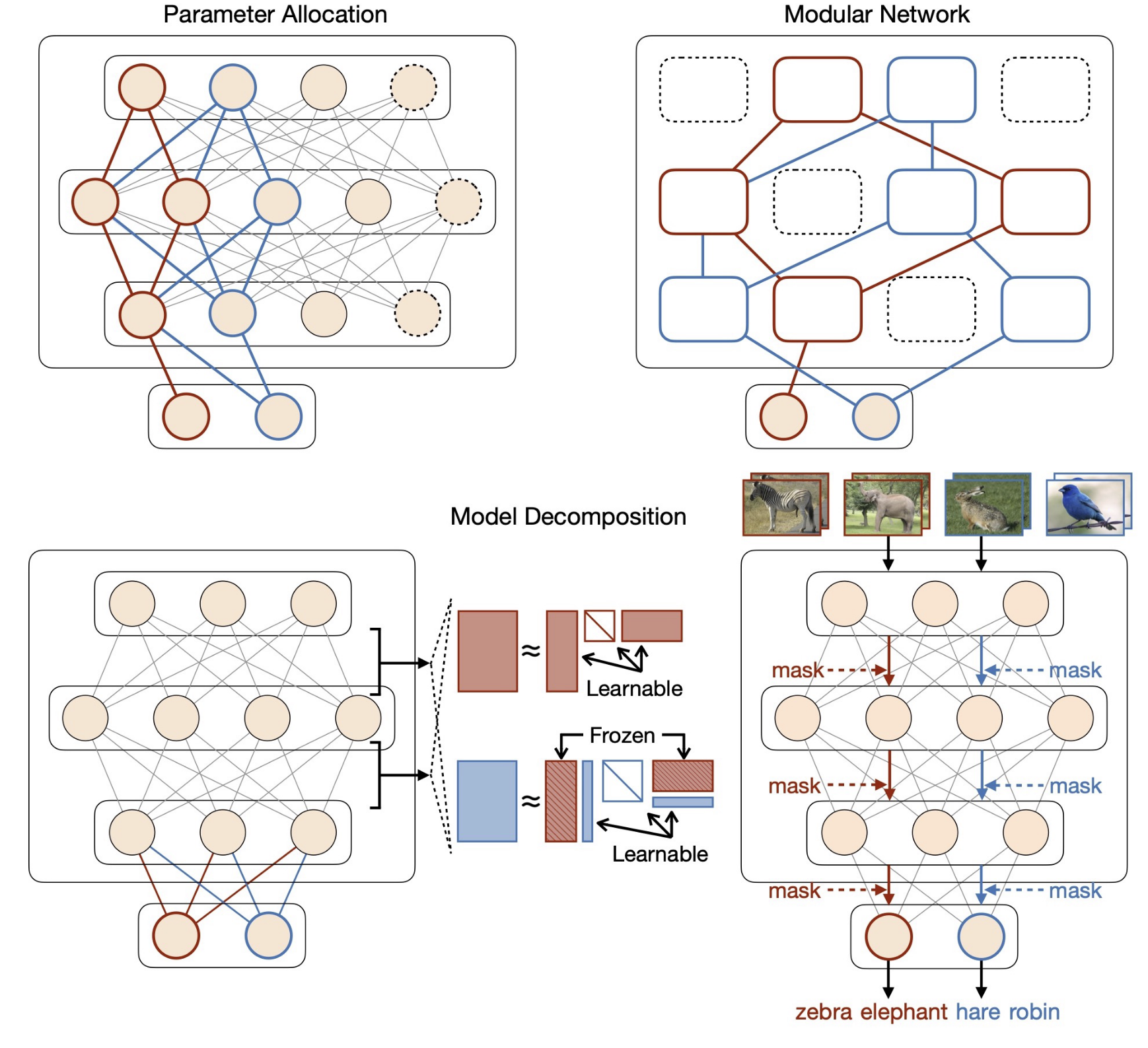
While the replay and regularisation-based approaches try to escape catastrophic forgetting on top of Finetuning by their forgetting preventing mechanisms, architecture-based approaches adopt distinctly different logic of strategy. These approaches leverages the separability characteristic of the neural network architecture. In other words, they treat the network as decomposable resources for tasks, rather than as a whole. The main idea is to dedicate different parts of a neural network to different tasks to minimize the inter-task interference.

The “part” of a network can be regarded in various ways, which leads to different kinds of architecture-based approaches.

• Modular networks: play around network modules like layers, blocks. The basic “part” unit is module.
• Parameter allocation: allocate group of parameters or neurons to task as subnet. The basic “part” unit is parameter or neuron.
• Model decomposition: decompose network from various aspects into shared and task-specific components. The component could be any part of the machine learning systems like modules itself, or a mathematical decomposition of each parameters. The basic “part” unit is the component that the approach decomposes the model into.

Three ways of decomposing neural network into parts in architecture-based approaches. (Source: L. Wang et al. 2024)

I have another post that introduces many architecture-based approaches in detail: Architecture-Based Continual Learning Algorithms.

The challenge of network capacity (challenge 3 in Section 3.6) becomes very explicit in architecture-based approaches, because the “parts” of the network they decompose are direct reflection of the network capacity.

Many architecture-based approaches naturally fix the subnet allocated for previous tasks, which is the best way to prevent forgetting (some paper even says they have achieved zero forgetting, but yeah that’s true), and gives maximum stability to the continual learning model. However, as we have discussed above, if the approach does everything within a fixed network, the capacity will eventually reach its limit. At this point, the model faces a big low plasticity problem. Therefore, a lot of architecture-based approaches allow expanding the network to get extra capacity when needed from nowhere, which is criticised unfair.

4.4 Optimisation-based Approaches

Optimisation-based approaches directly manipulate the explicit optimisation step during training of new task. We are not talking about the loss function, which we have discussed in regularisation-based approaches and is considered as less direct optimisation manipulation. The more direct manipulation, here in optimisation-based approaches, often involves modification of the gradients from $g$ calculated from the classification loss to $g^{\prime }$, then use $g^{\prime }$ for the gradient descent step.

To be specific, A common strategy is to project the gradient $g$ onto a new direction that avoids conflicts with the objectives of previous tasks. Since updating along parallel directions could disrupt earlier tasks, many approaches choose to use orthogonal directions as the new direction.

For example, OGD (Orthogonal Gradient Descent) (Farajtabar et al. 2020) preserves a key gradient direction for each previous task and project the gradient orthogonal onto it when training new task. In theory, that key gradient should be the current model’s gradients calculated with respect to the data from previous tasks, but we have no access to previous data after their training. To address this, OGD employs an empirical approximation, such as saving the average gradients that were calculated during the training of the previous tasks as the key gradient.

Tip

If you know linear algebra, the projected orthogonal direction of given directions can be calculated by the Gram-Schmidt formula.

You might wonder whether there is enough space to accommodate multiple gradients orthogonally. The answer is yes, because neural network operates in a high-dimensional parameter space, which is typically much larger than or at least comparable to the number of data points. In such a high-dimensional space, there will always be directions where gradients can be orthogonally aligned without conflict.

5 Present and Future

Continual learning was quite popular from around 2018 to 2022, but it seems to have experienced a decline in attention in recent years. During this period, researchers shifted their focus to applying the concept of continual learning to other popular paradigms, leading to the development of approaches like Few-Shot Continual Learning (FSCL), Unsupervised Continual Learning (UCL), Online Continual Learning (OCL), etc, which were sometimes regarded as paper mills 😂. However, AI has also seen rapid advancements in technologies like self-supervised learning and LLMs (large language models) in recent years. They have opened up new opportunities for continual learning and leads to many significant works using them. In this section, I’m going to discuss this trend and the notable works, which are the actual pathways to publish continual learning papers if you decide to dive into this field.

5.1 Continual Learning + Self-Supervised Learning

Some works design special network architectures and use representation learning techniques to learn meaningful representations for each task, which are then leveraged to prevent forgetting. These techniques often involve self-supervised learning (SSL), such as contrastive learning.

Self-supervised learning offers its own advantages. First, it enables the model to learn representations that generalize well, which is crucial for continual learning and helps prevent forgetting. For example, DualNet (Pham, Liu, and Hoi 2021) introduces the idea of dividing the network into “fast” and “slow” components, corresponding to task-specific and shared representations. They use the self-supervised loss called Barlow Twins (Zbontar et al. 2021) for the slow network, which encourages more generalizable features.

Second, many SSL techniques are effective tools for promoting specific goals in representation learning. For instance, contrastive loss forces the model to generate similar representations for samples deemed similar, and dissimilar representations for contrastive samples. This is particularly useful in continual learning if we want to contrast representations of new and previous tasks, we ensure they are kept distinct in the representation space, which is exactly what we need to prevent forgetting. This is the core idea behind Co2L (Contrastive Continual Learning) (Cha, Lee, and Shin 2021), the pioneering work that combines contrastive learning with continual learning.

5.2 Continual Learning + Pre-train Models

Large pre-trained models have gained significant popularity since 2018, with models from BERT to GPT, bringing transformative changes to AI research and even to our daily lives. Continual learning has also been benefiting from these most popular advances.

Some works leverage pre-trained models as a shared knowledge base across tasks in continual learning. This approach is straightforward: pre-trained models already create powerful representations, so all we need to do is fine-tune them for each specific task. The concept of pre-training fits naturally into continual learning.

However, as model sizes continue to grow in the course of AI research, full fine-tuning has become increasingly computationally expensive, which also affects the feasibility of continual learning. This led to the rise of prompt-based learning around 2020, which quickly gained popularity. In this approach, researchers don’t fine-tune the entire model with updating the parameters; instead, they design specific prompts that “guide” the model to use its pre-trained knowledge for particular tasks, which act like a plugin the pre-trained model base without updating the parameters. As we know, the update of parameters is the direct cause of forgetting, thereby this technique that doesn’t even need to update parameters becomes a black magic for continual learning.

To apply this method to continual learning, the question now becomes how to generate task-specific prompts from the data. Currently, one simple approach is to select the most relevant prompts from a pre-defined prompt pool. For instance, the leading work L2P (Learning to Prompt for Continual Learning) (Z. Wang et al. 2022) introduces an instance-wise query mechanism, where the ideal prompt is retrieved based on the specific instance. This instance-wise approach doesn’t require knowledge of the task ID, making it well-suited for task-agnostic testing.

Some works have also proposed making the pre-training process itself continuous, which are referred to as CPT (Continual Pre-training). They believe that the approaches mentioned earlier do not address the fundamental issue, as large models themselves are typically pre-trained in an incremental manner thus require continual learning. They emphasize that performing upstream continual learning to improve downstream performance is particularly crucial from a practical perspective.

6 Resources Centre

Other Posts:

1. A Summary of Continual Learning Metrics
2. Architecture-Based Continual Learning Algorithms

Slides:

1. Architecture-Based Approaches in Continual Learning
2. Learning with Non-Stationary Streaming Data: A Beginner’s Guide to Continual Learning

References

Cha, Hyuntak, Jaeho Lee, and Jinwoo Shin. 2021. “Co2l: Contrastive Continual Learning.” In Proceedings of the IEEE/CVF International Conference on Computer Vision, 9516–25.

De Lange, Matthias, Rahaf Aljundi, Marc Masana, Sarah Parisot, Xu Jia, Aleš Leonardis, Gregory Slabaugh, and Tinne Tuytelaars. 2021. “A Continual Learning Survey: Defying Forgetting in Classification Tasks.” IEEE Transactions on Pattern Analysis and Machine Intelligence 44 (7): 3366–85.

Farajtabar, Mehrdad, Navid Azizan, Alex Mott, and Ang Li. 2020. “Orthogonal Gradient Descent for Continual Learning.” In International Conference on Artificial Intelligence and Statistics, 3762–73. PMLR.

Hemati, Hamed, Marco Schreyer, and Damian Borth. 2021. “Continual Learning for Unsupervised Anomaly Detection in Continuous Auditing of Financial Accounting Data.” arXiv Preprint arXiv:2112.13215.

Kirkpatrick, James, Razvan Pascanu, Neil Rabinowitz, Joel Veness, Guillaume Desjardins, Andrei A Rusu, Kieran Milan, et al. 2017. “Overcoming Catastrophic Forgetting in Neural Networks.” Proceedings of the National Academy of Sciences 114 (13): 3521–26.

Lesort, Timothée, Vincenzo Lomonaco, Andrei Stoian, Davide Maltoni, David Filliat, and Natalia Dı́az-Rodrı́guez. 2020. “Continual Learning for Robotics: Definition, Framework, Learning Strategies, Opportunities and Challenges.” Information Fusion 58: 52–68.

Li, Zhizhong, and Derek Hoiem. 2017. “Learning Without Forgetting.” IEEE Transactions on Pattern Analysis and Machine Intelligence 40 (12): 2935–47.

Liu, Shu, Bo Wang, Huaxiong Li, Chunlin Chen, and Zhi Wang. 2023. “Continual Portfolio Selection in Dynamic Environments via Incremental Reinforcement Learning.” International Journal of Machine Learning and Cybernetics 14 (1): 269–79.

Pham, Quang, Chenghao Liu, and Steven Hoi. 2021. “Dualnet: Continual Learning, Fast and Slow.” Advances in Neural Information Processing Systems 34: 16131–44.

Rebuffi, Sylvestre-Alvise, Alexander Kolesnikov, Georg Sperl, and Christoph H Lampert. 2017. “Icarl: Incremental Classifier and Representation Learning.” In Proceedings of the IEEE Conference on Computer Vision and Pattern Recognition, 2001–10.

Shaheen, Khadija, Muhammad Abdullah Hanif, Osman Hasan, and Muhammad Shafique. 2022. “Continual Learning for Real-World Autonomous Systems: Algorithms, Challenges and Frameworks.” Journal of Intelligent & Robotic Systems 105 (1): 9.

Singh, Tinku, Riya Kalra, Suryanshi Mishra, Satakshi, and Manish Kumar. 2023. “An Efficient Real-Time Stock Prediction Exploiting Incremental Learning and Deep Learning.” Evolving Systems 14 (6): 919–37.

Van de Ven, Gido M, and Andreas S Tolias. 2019. “Three Scenarios for Continual Learning.” arXiv Preprint arXiv:1904.07734.

Verwimp, Eli, Kuo Yang, Sarah Parisot, Lanqing Hong, Steven McDonagh, Eduardo Pérez-Pellitero, Matthias De Lange, and Tinne Tuytelaars. 2023. “Clad: A Realistic Continual Learning Benchmark for Autonomous Driving.” Neural Networks 161: 659–69.

Wang, Liyuan, Xingxing Zhang, Hang Su, and Jun Zhu. 2024. “A Comprehensive Survey of Continual Learning: Theory, Method and Application.” IEEE Transactions on Pattern Analysis and Machine Intelligence.

Wang, Zifeng, Zizhao Zhang, Chen-Yu Lee, Han Zhang, Ruoxi Sun, Xiaoqi Ren, Guolong Su, Vincent Perot, Jennifer Dy, and Tomas Pfister. 2022. “Learning to Prompt for Continual Learning.” In Proceedings of the IEEE/CVF Conference on Computer Vision and Pattern Recognition, 139–49.

Zbontar, Jure, Li Jing, Ishan Misra, Yann LeCun, and Stéphane Deny. 2021. “Barlow Twins: Self-Supervised Learning via Redundancy Reduction.” In International Conference on Machine Learning, 12310–20. PMLR.