Architecture-Based Continual Learning Algorithms

In this post, I’m diving into details about architecture-based approaches. If you are new to continual learning, please check out my continual learning beginners’ guide and its architecture-based approach chapter first.

Slides for this post: Architecture-Based Approaches in Continual Learning

Just to recap, we divide architecture-based algorithms into 3 categories, based on a recent survey paper (L. Wang et al. 2024):

1. Modular Networks
2. Parameter Allocation
3. Model Decomposition

We will go through the algorithms in each category, and compare them from certain perspectives at the end.

Category 1: Modular Networks

When we implement neural networks in any programming frameworks, we always find the networks composed from modules. They could be linear or convolution layers, a block of layers, decoders or encoders, or anything. In this category of modular networks, we play around the modules.

Progressive Networks

Progressive networks (Rusu et al. 2016), one of the earliest works in continual learning, simply expands the network each time a new task arrives, and allocates this new part to the new task. In Figure 1, an equal-sized set of modules (one column in the figure) is initialised for the new task. When training the new task, only the newly introduced parameters (solid arrows) are updated while previous parameters (dashed arrows) are fixed. The original paper (like “output1, 2, 3” illustrated in the figure) indicates it can only be applied to task incremental learning (TIL).

Figure 1: Progressive Networks. (Source: Rusu et al. 2016)

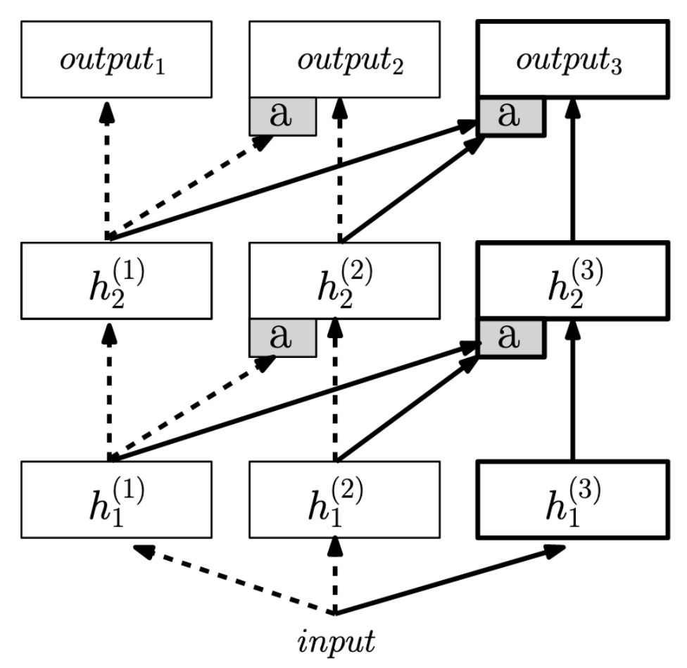
This method is simple and very effective, but at the huge cost of linearly growing network size. The network size is proportional to the number of tasks, which is absolutely not scalable in the long run.

Note

You would probably say it is the same as independent learning; yes that’s true, and it is actually a bit further than independent learning because it has the parameters from previous task parts to new task part (the upper right arrows).

Expert Gate

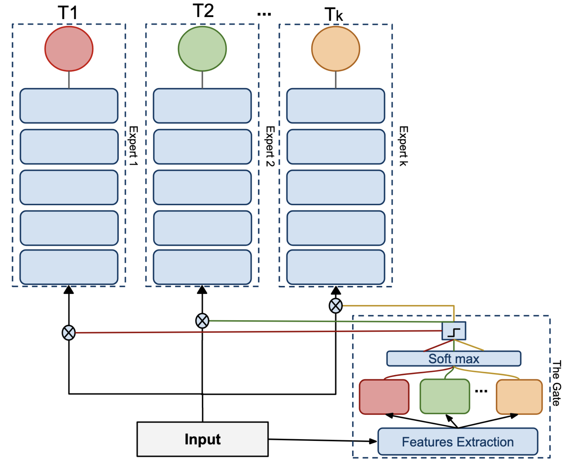
Expert Gate (Aljundi, Chakravarty, and Tuytelaars 2017) is another early approach of linear expanded network (called “experts” in the paper) and expansions are independent in terms of architecture without parameters connecting. This seems not even smarter than independent learning, but their main contribution is that it works in the task-agnostic testing where task IDs of test instances are unknown so the model has to figure them out by itself. In this approach, a gate works as the task ID selector at test time, which is also a network learned through the task sequence.

Figure 2: Expert Gate. (Source: Aljundi, Chakravarty, and Tuytelaars 2017)

PathNet

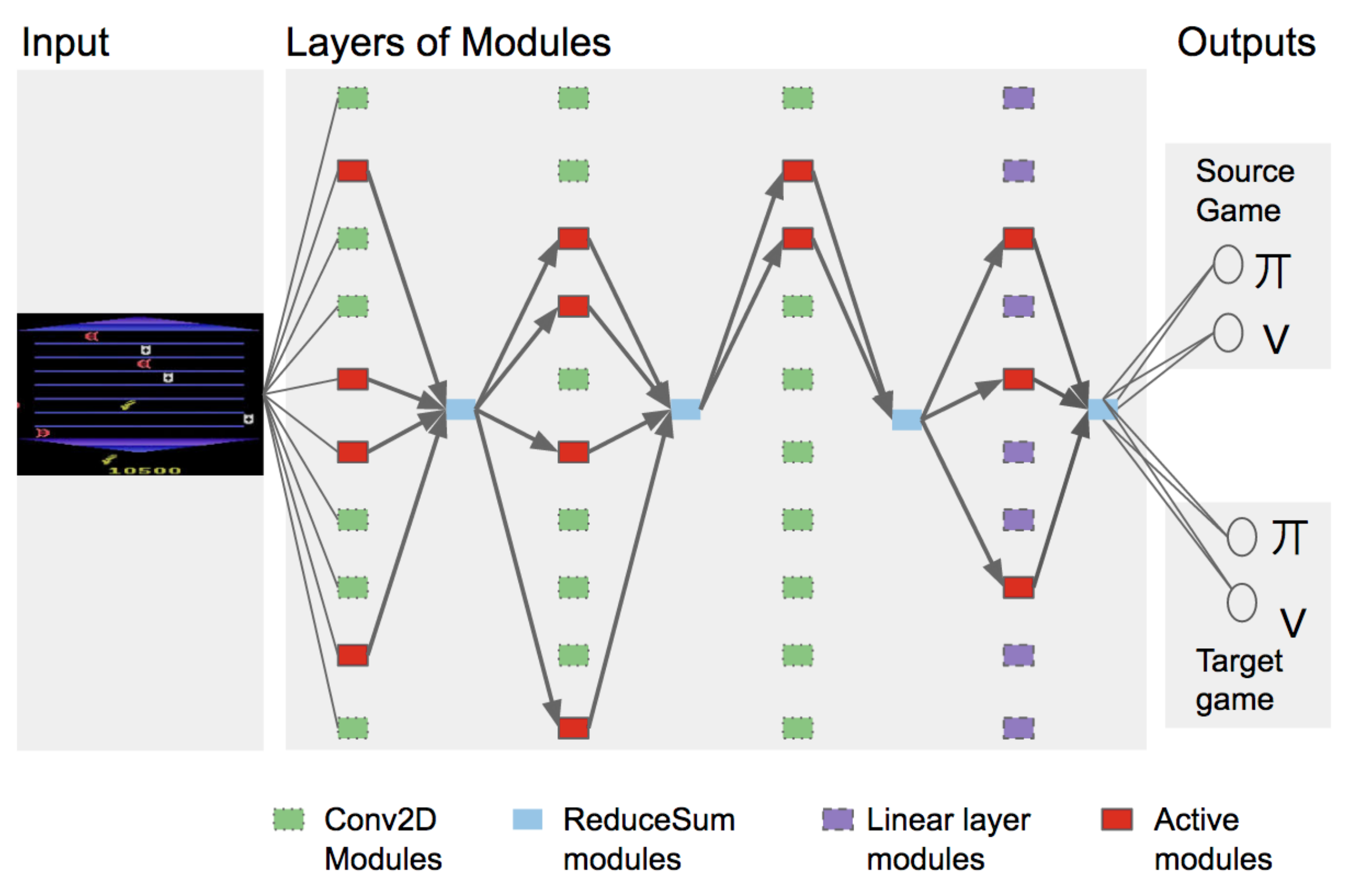
Some work does not expand the network at all. PathNet (Fernando et al. 2017) prepares a large pool of modules for the algorithm to select from. For each position in the module sequence, several options are provided (each column in Figure 3). The selected modules are contacted as a subnet (called “path” in the paper) that each task corresponds to from the huge network. The selection strategy is genetic algorithm, involving tournaments between different paths during the training of a task.

Figure 3: PathNet. (Source: Fernando et al. 2017)

Category 2: Parameter Allocation

The above method of dissecting the network to modules can be refined to the level of parameters or neurons. Parameter allocation selects a set of parameters or neurons to allocate to each task. They can also form a subnet of the network.

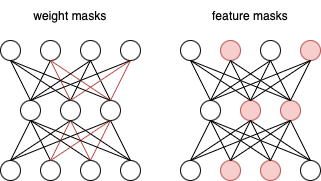
The selection of a parameter or neuron can be represented as a binary mask value. Collectively, the mask values can be represented as mask vectors or matrices. Figure 4 shows the two ways to select a subnet of a network: weight masks on parameters, and feature masks on neurons. Note that parameter masks could be incredibly greater in terms of scale (usually same as parameter space), and that’s why most works adopt the feature masks.

Figure 4: An illustration of weight and feature masks.

Warning

The algorithm should ensure that a balanced number of parameters or neurons are selected to form a proper subnet in each layer. We don’t want to see a disconnected subnet or a subnet with some 1-dimensional hidden layer.

The parameter allocation approaches vary in terms of:

• Allocation strategies: some assign masks through manual rules, some learn the masks during training.
• How masks are applied during training: masks can potentially be used to select forward pass, backward pass, and parameter update step during training. Most methods fix the selected subnet after trained on corresponding task and use it as the only model to predict for that task during testing.

PackNet

PackNet (Mallya and Lazebnik 2018) represents the most naive way to do parameter allocation. It:

• Uses a fixed network;
• Uses weight masks;
• Selected subnets are not overlapped;
• Allocates subnets (i.e. select weights for a task) by manual rules.

It trains the entire unallocated part of the network for the new task with the subnet for previous tasks fixed, and use a selection strategy to prune and reserve the weights out of the part for the new task. (After pruning, a bit retraining is needed since the model for the task has changed.)

Figure 5: PackNet. (Source: Mallya and Lazebnik 2018)

The weight selection (pruning) strategy is post-hoc and based on value filtering. It simply selects a fixed percentage of weights with top absolute value and prunes the rest. This strategy believes that the weights with greater absolute values are more important.

This manual way of allocation brings up a big problem. It’s known for sure how much network capacity is available after training each task, and this depends solely on the pruning rate hyperparameter. For example, the pruning rate is set as 60% in Figure 5, so we can expect for sure that after 3 tasks the network has ${0.6}^3=21.6\mathrm{\%}$ of the original capacity. Therefore, PackNet is completely non-adaptive and non-dynamic.

Also, we can find that the network capacity can run out quickly after a fixed number of tasks. Since the network is fixed, and subnet is fixed once trained and allocated to task in this approach, it provides a obvious example of what we mentioned in the continual learning beginners’ guide that the network capacity is a big issue in architecture-based approaches.

DEN

DEN (Dynamically Expandable Networks) (Yoon et al. 2017) is a parameter allocation approach that:

• Dynamically expands the network;
• Uses feature masks;
• Selected subnets can be overlapped;
• Allocates subnets (i.e. select neurons for a task) in a less manual way, but still controlled by hyperparameters.

This work has several highlights. First, it expands the network in a dynamic way rather than keep expanding every new task linearly whenever new task arrives like Progressive Networks and Expert Gate do. The network only expands when needed – when the loss can’t meet a certain threshold.

Second, the selection strategy is interesting. It leverages the idea of regularisation-based approaches, but for the purpose of selecting neurons. In this work, you can find training with L1 regularisation that aims to get sparse parameters thus naturally complete the selection work. You can also find another selection strategy that leverages L2 regularisation indirectly. We have discussed L2 regularisation in the continual learning guide post, and we know that it equally penalises all parameters to be close to previous learned ones. However, regularisation is always a soft constraint, thus the parameters still updates. At this time, parameters that change more are considered to be important, thus selected.

Figure 6: DEN (Dynamically Expandable Networks). (Source: Yoon et al. 2017)

As we can see, this work combines many ideas, so it naturally has many hyperparameters to tune, like the threshold $\tau$ for loss and the threshold $\sigma$ for parameter change. This makes it a very complicated system.

Piggyback & SupSup

One way is to make allocation adaptive is to learn masks during training. In this case, masks are treated learnable parameters, just like model parameters. However, the main problem is that masks are binary, not real values, thus not differentiable.

Piggyback is the first work to treat binary masks as mapped from real values through a gate function (like Sigmoid), and train the real values that are differentiable. It uses weight masks.

However, this work doesn’t allow the network parameters to be trained. In other words, the backbone network is a fixed knowledge base that only allows selecting subnet from it. This certainly reduces representation ability, but we can imagine that if we use a large pre-trained network as the backbone, it would probably be fine.

Figure 7: Piggyback. (Source: Mallya, Davis, and Lazebnik 2018)

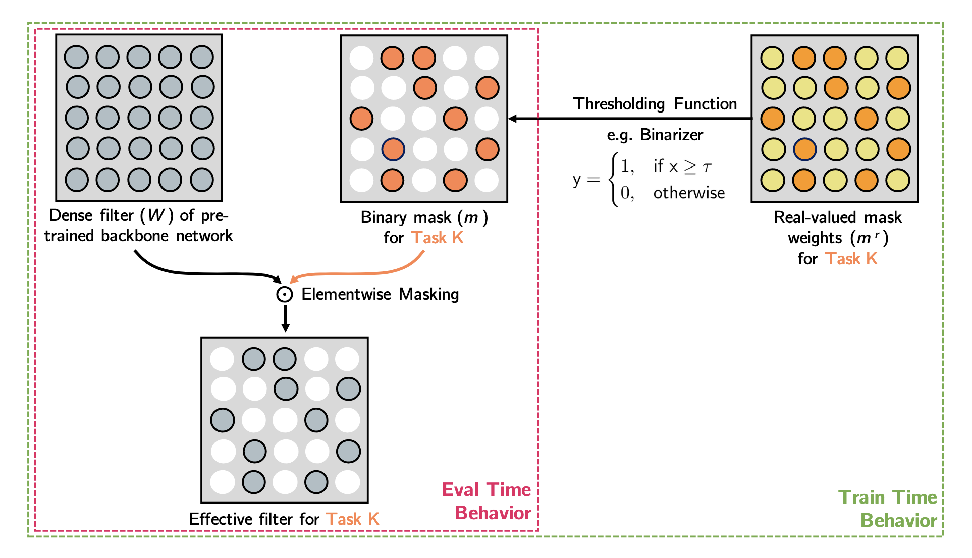
Another work called SupSup (Wortsman et al. 2020) extends Piggyback to task-agnostic testing paradigm. I won’t go into details.

HAT & AdaHAT

HAT (Hard Attention to the Task) (Serra et al. 2018) also uses learnable masks mapped from real values (called task embeddings in the paper) to allocate, but allows the network parameters to be trained. It uses feature masks. It is a good example of adaptive allocation.

However, HAT, like PackNet, uses fixed network and fixed the subnet once trained and allocated to task, also suffers from network capacity problem. In order to alleviate this, it proposed a regularisation to promote the task embeddings sparse from the unallocated part of the network. This is a good idea, but it can only slow down the speed of capacity exhaustion, which is still not enough to solve the problem.

Figure 8: HAT and AdaHAT. (Source: P. Wang et al. 2024)

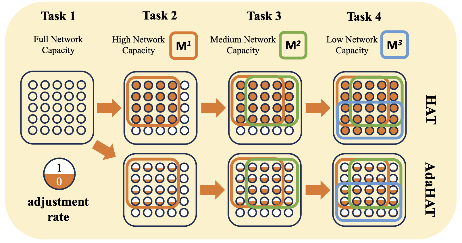
My work AdaHAT (Adaptive Hard Attention to the Task) (P. Wang et al. 2024) aims to recycle less important network capacity by allowing updates to the subnet after trained on previous tasks. The intensity of the updates is designed to be determined by some heuristic indicators, such as parameter importance and current capacity usage. The network is able to manage its own capacity in an adaptive way, without the need for many manual hyperparameters, and alleviate the capacity problem to a large extent.

CPG

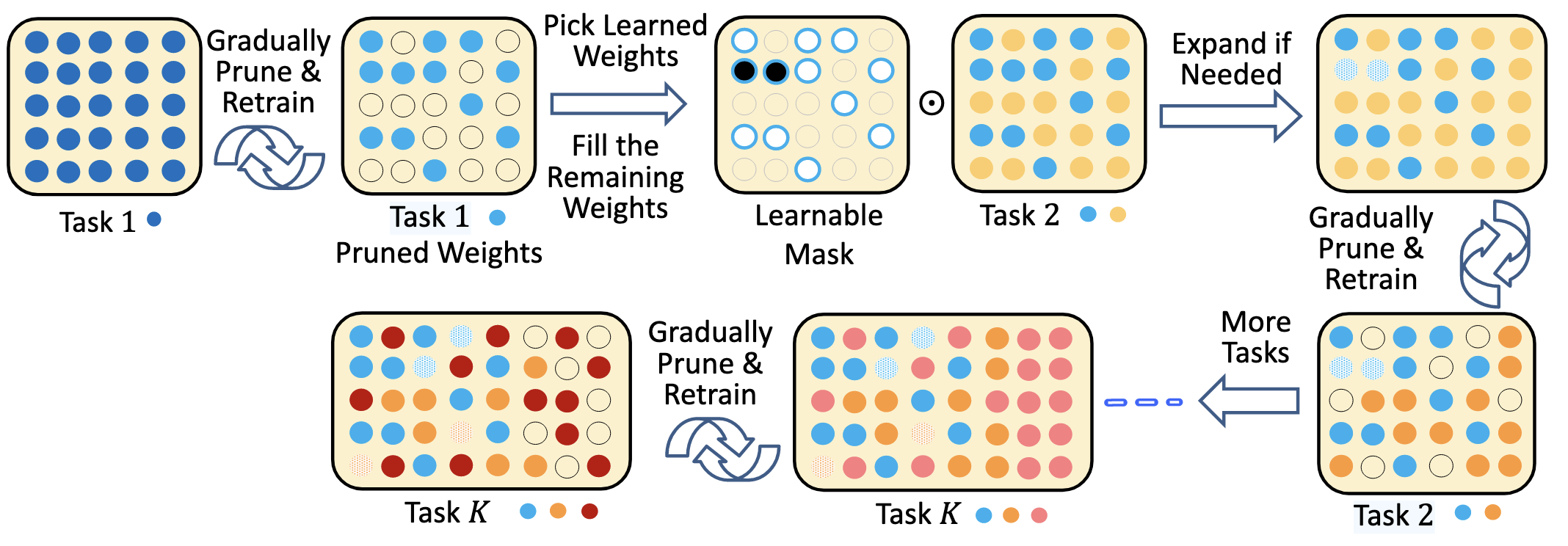
CPG (Compacting, Picking and Growing) (Hung et al. 2019) is a complicated system combining the ideas mentioned above: post-hoc pruning (called “compacting”) and retraining, learnable masks (called “picking”), network expansion (called “growing”).

Figure 9: CPG (Compacting, Picking and Growing). (Source: Hung et al. 2019)

Category 3: Model Decomposition

A neural network can not only be decomposed equally through its architecture in terms of parameters and neurons, but also other ways and even other forms of components, which model decomposition approaches explore.

The typical way that this category of approaches does is to divide the network into shared (task-agnostic) and task-specific parts, where a task is associated with both shared and its specific parts. This idea works fine but still has a growing memory problem like network expansion. Task-specific parts grow linearly with the number of tasks, even though the shared part is fixed.

ACL

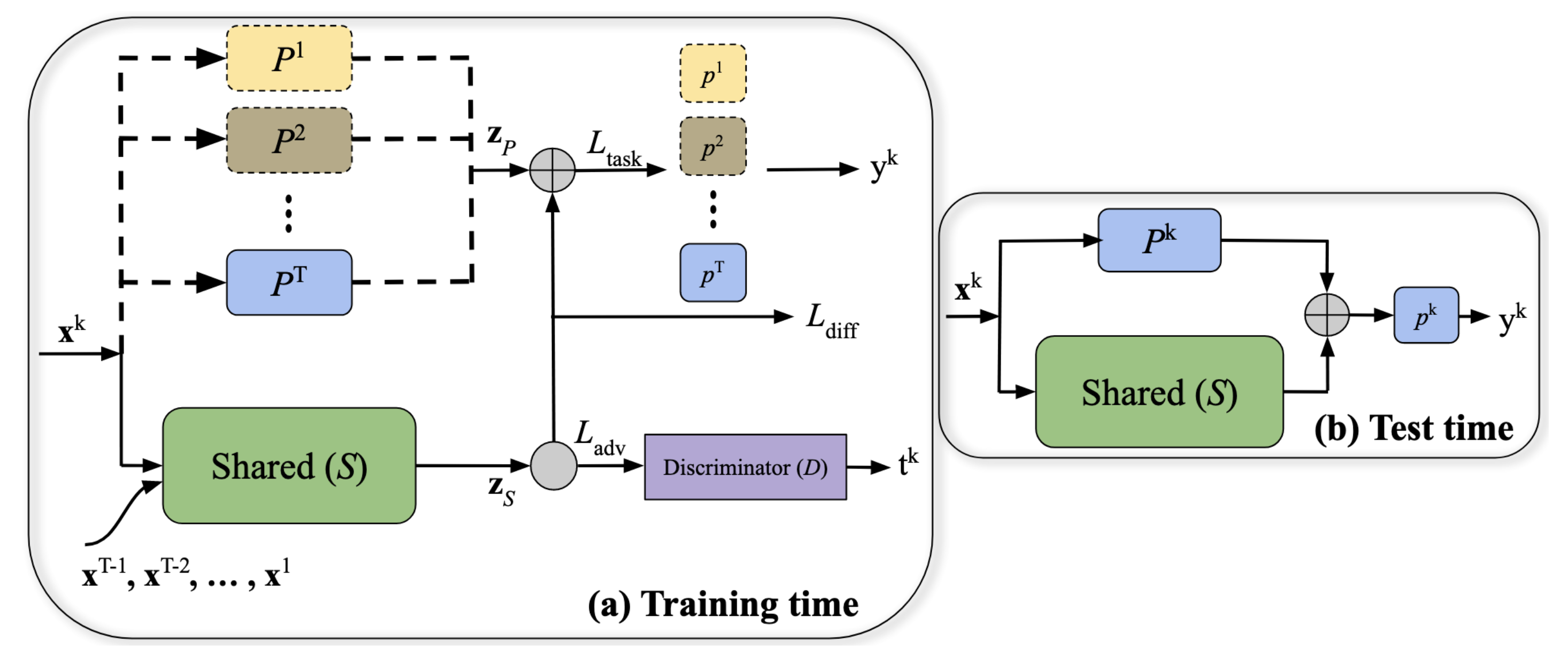
ACL (Adversial Continual Learning) (Ebrahimi et al. 2020) divide the network into shared and task-specific parts in terms of architecture, like Figure 10 shows. The parts have different objectives:

• The shared part is trained to be task-agnostic. This approach uses adversarial loss that are generally used to encourage model robustness and generalisation ability in deep learning research;
• The task-specific part is trained to be task-specific, thus conventional classification loss is used.
• A “difference” loss is applied additionally to encourage distinction between shared and task-specific parts, by preventing shared features appearing in task-specific part.

Figure 10: ACL (Adversial Continual Learning). (Source: Ebrahimi et al. 2020)

APD

APD decomposes the parameters mathematically into shared and task-specific parameters. Given a parameter matrix ${\theta }_t$ of a layer, it is decomposed as the following way:

$${\theta }_t=\sigma \odot {\mathbf{M}}_t+{\tau }_t$$

Here $\sigma$ denotes the shared parameters, ${\mathbf{M}}_t$ and ${\tau }_t$ are the task-specific parameters. They also have different objectives, treated in different ways by the algorithm:

• The shared parameters are trained to be task-agnostic. This approach uses L2 regularisation (on parameter change) to encourage shared parameters to be close to what it has learned before;
• The task-specific parameters are trained to be task-specific. This approach uses L1 regularisation (on parameter value itself) to encourage task-specific parameters to be sparse;
• Apart from them, the shared and task-specific parameters are together trained with the conventional classification loss.

Comparison

We now compare the architecture-based algorithms from these perspectives:

• Whether the network is fixed;
• Whether the “parts” for different tasks are allowed overlapped.

Approach	Category	Fixed Network?	Allow Overlap?
Progressive Networks	Modular Networks	No	Yes
Expert Gate	Modular Networks	No	Yes
PathNet	Modular Networks	Yes	No
PackNet	Parameter Allocation	Yes	Yes
DEN	Parameter Allocation	No	No
Piggyback	Parameter Allocation	Yes	No
HAT	Parameter Allocation	Yes	No
WSN	Parameter Allocation	Yes	No
-	Model Decomposition	No	No

References

Aljundi, Rahaf, Punarjay Chakravarty, and Tinne Tuytelaars. 2017. “Expert Gate: Lifelong Learning with a Network of Experts.” In Proceedings of the IEEE Conference on Computer Vision and Pattern Recognition, 3366–75.

Ebrahimi, Sayna, Franziska Meier, Roberto Calandra, Trevor Darrell, and Marcus Rohrbach. 2020. “Adversarial Continual Learning.” In Computer Vision–ECCV 2020: 16th European Conference, Glasgow, UK, August 23–28, 2020, Proceedings, Part XI 16, 386–402. Springer.

Fernando, Chrisantha, Dylan Banarse, Charles Blundell, Yori Zwols, David Ha, Andrei A Rusu, Alexander Pritzel, and Daan Wierstra. 2017. “Pathnet: Evolution Channels Gradient Descent in Super Neural Networks.” arXiv Preprint arXiv:1701.08734.

Hung, Ching-Yi, Cheng-Hao Tu, Cheng-En Wu, Chien-Hung Chen, Yi-Ming Chan, and Chu-Song Chen. 2019. “Compacting, Picking and Growing for Unforgetting Continual Learning.” Advances in Neural Information Processing Systems 32.

Mallya, Arun, Dillon Davis, and Svetlana Lazebnik. 2018. “Piggyback: Adapting a Single Network to Multiple Tasks by Learning to Mask Weights.” In Proceedings of the European Conference on Computer Vision (ECCV), 67–82.

Mallya, Arun, and Svetlana Lazebnik. 2018. “Packnet: Adding Multiple Tasks to a Single Network by Iterative Pruning.” In Proceedings of the IEEE Conference on Computer Vision and Pattern Recognition, 7765–73.

Rusu, Andrei A, Neil C Rabinowitz, Guillaume Desjardins, Hubert Soyer, James Kirkpatrick, Koray Kavukcuoglu, Razvan Pascanu, and Raia Hadsell. 2016. “Progressive Neural Networks.” arXiv Preprint arXiv:1606.04671.

Serra, Joan, Didac Suris, Marius Miron, and Alexandros Karatzoglou. 2018. “Overcoming Catastrophic Forgetting with Hard Attention to the Task.” In International Conference on Machine Learning, 4548–57. PMLR.

Wang, Liyuan, Xingxing Zhang, Hang Su, and Jun Zhu. 2024. “A Comprehensive Survey of Continual Learning: Theory, Method and Application.” IEEE Transactions on Pattern Analysis and Machine Intelligence.

Wang, Pengxiang, Hongbo Bo, Jun Hong, Weiru Liu, and Kedian Mu. 2024. “AdaHAT: Adaptive Hard Attention to the Task in Task-Incremental Learning.” In Joint European Conference on Machine Learning and Knowledge Discovery in Databases, 143–60. Springer.

Wortsman, Mitchell, Vivek Ramanujan, Rosanne Liu, Aniruddha Kembhavi, Mohammad Rastegari, Jason Yosinski, and Ali Farhadi. 2020. “Supermasks in Superposition.” Advances in Neural Information Processing Systems 33: 15173–84.

Yoon, Jaehong, Eunho Yang, Jeongtae Lee, and Sung Ju Hwang. 2017. “Lifelong Learning with Dynamically Expandable Networks.” arXiv Preprint arXiv:1708.01547.