AI Concept Takeaway: Recurrent Neural Networks (RNN)

My takeaway series follow a Q&A format to explain AI concepts at three levels:

TipConceptual Level

Anyone with general knowledge can understand them.

WarningImplementation Level

For anyone who wants to dive into the code implementation details of the concept.

ImportantMathematical Level

For anyone who wants to understand the mathematics behind the technique.

---

TipWhat is Recurrent Neural Network (RNN)?

Recurrent Neural Network (RNN) is a type of neural network designed for processing sequential data. Unlike conventional neural networks that take single input to single output, RNNs have connections that loop back on themselves (which is recurrent), allowing accumulating information over the sequential data iteratively.

TipWhy do we need RNN for sequential data, instead of feeding them into conventional neural networks?

Because RNNs can naturally handle variable-length sequential data. If we feed sequential data into conventional neural networks, we have to fix the length of the input sequence, either by truncating longer sequences or padding shorter ones. This can lead to loss of information or introduce noise.

ImportantWhat are the inputs and outputs of vanilla RNN?

The RNN processes sequences of data.

Inputs:

• A sequence of input data ${\mathbf{x}}_1,{\mathbf{x}}_2,\dots ,{\mathbf{x}}_T$ of any length, where $T$ is the length of the sequence. The index $t$ is called the time step in the sequence.

Outputs:

• A sequence of outputs ${\mathbf{y}}_1,{\mathbf{y}}_2,\dots ,{\mathbf{y}}_T$ of the same length as the input sequence, where each output ${\mathbf{y}}_t$ corresponds to the input at time step $t$.

Please note, a RNN can receive any length of sequence. The length $T$ can vary between different input data fed into the RNN.

ImportantWhat is the architecture of vanilla RNN?

The vanilla RNN architecture is illustrated as follows:

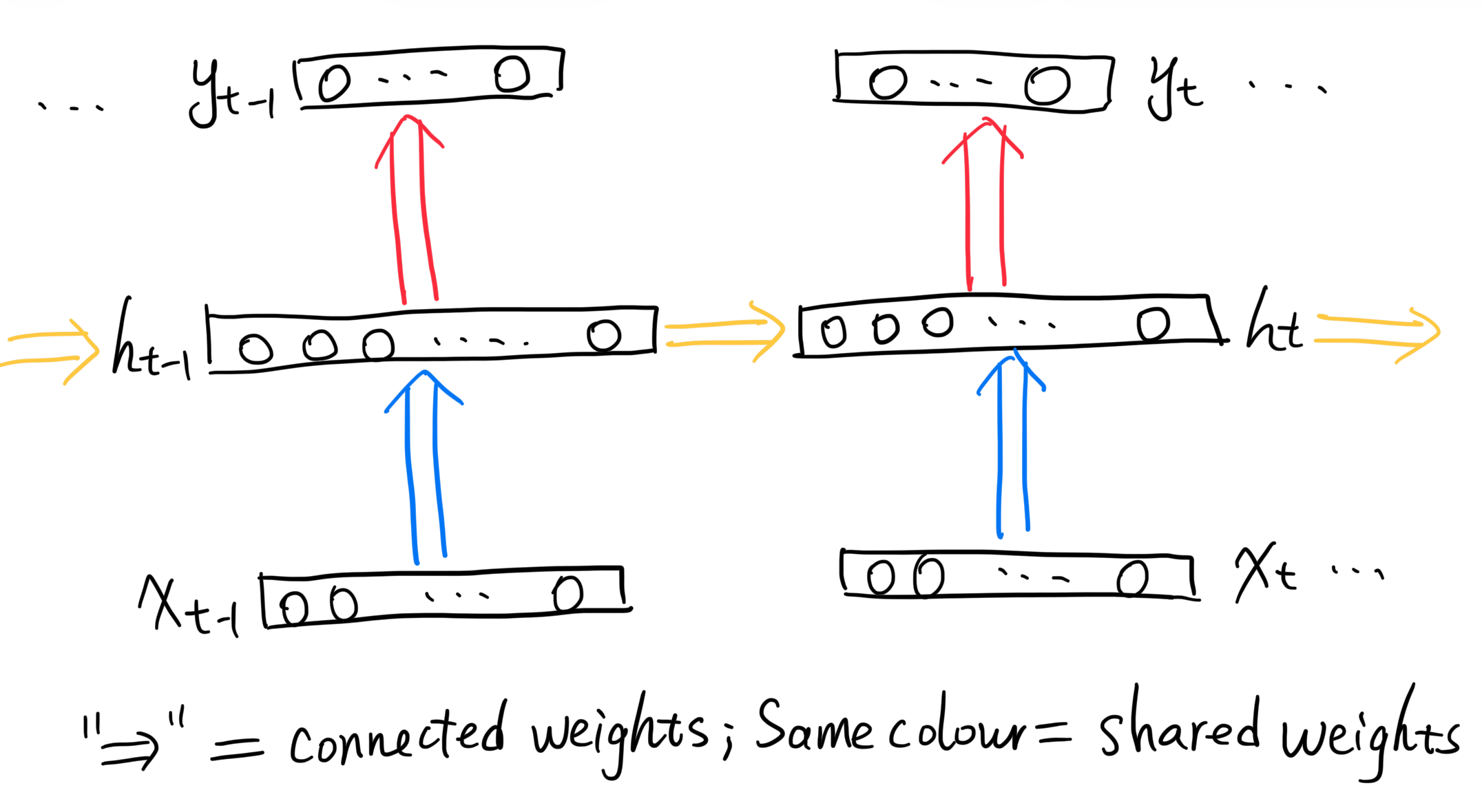
The blue and yellow arrows are the connections between the input and hidden states:

$$\begin{array}{}\text{(1)}& {\mathbf{h}}_t=f({\mathbf{W}}_{xh}{\mathbf{x}}_t+{\mathbf{W}}_{hh}{\mathbf{h}}_{t-1}+{\mathbf{b}}_h)\end{array}$$

The red arrow is the connection between the hidden state and output:

$$\begin{array}{}\text{(2)}& y_t=g({\mathbf{W}}_{hy}{\mathbf{h}}_t+{\mathbf{b}}_y)\end{array}$$

These weights are shared across all time steps, which is a key feature of RNNs that allows them to generalise across different sequence lengths.

ImportantWhat is the forward pass of RNN?

The forward pass of RNN involves iterating through each time step of the input sequence and updating the hidden state and output at each step, instead of processing the entire sequence at once.

1. Hidden state initialization: Set the initial hidden state ${\mathbf{h}}_0$ to a vector of zeros or random values.
2. For each time step $t$ from $1$ to $T$:
   • Compute the new hidden state ${\mathbf{h}}_t$ using the current input ${\mathbf{x}}_t$ and the previous hidden state ${\mathbf{h}}_{t-1}$ using Equation 1.
   • Compute the output $y_t$ using the current hidden state ${\mathbf{h}}_t$ using Equation 2.

TipWhat is the hidden state for?

The hidden state ${\mathbf{h}}_t$ serves not only as a hidden layer in the neural network, but also as a memory that captures information about the sequence up to time step $t$ because it iterates itself through the sequence. It allows the RNN to retain context from previous inputs, which is crucial for understanding sequential data where the meaning of an element can depend on its predecessors.

ImportantWhat is the backward pass of RNN?

The loss function of RNN is the average of the loss at each time step:

$$L=\frac{1}{T}\sum _{t=1}^T{L}_t(f({\mathbf{x}}_t;\theta ),y_t)$$

This is neither calculated and backpropagated at once, but step by step through time, which is called Backpropagation Through Time (BPTT):

1. For each time step $t$ from $1$ to $T$:
   • The forward pass computes the loss $L_t$ with respect to the output at each time step $t$.
   • The backward pass computes the gradients $\frac{\partial L_t}{\partial \theta }$ with respect to the model parameters $\theta =\{{\mathbf{W}}_{xh},{\mathbf{W}}_{hh},{\mathbf{W}}_{hy}\}$ (biases are ignored for simplicity) using the chain rule:
     • $\frac{\partial L_t}{\partial {\mathbf{W}}_{hy}}$ is first computed from differentiating Equation 2.
     • $\frac{\partial L_t}{\partial {\mathbf{W}}_{hh}}$ is then computed from differentiating Equation 1. Because this part of forward pass involves a chain ${\mathbf{h}}_0,\cdots ,{\mathbf{h}}_t$, it will backpropagate through all the hidden states from time step $t$ to $1$.
     • $\frac{\partial L_t}{\partial {\mathbf{W}}_{xh}}$ is also computed from differentiating Equation 1. This is done after backpropagating through all the hidden states from time step $t$ to $1$.
2. The total gradient is the sum of the gradients from each time step:

$$\frac{\partial L}{\partial \theta }=\sum _{t=1}^T\frac{\partial L_t}{\partial \theta }$$

TipWhat is RNN used for?

RNNs are commonly used for tasks involving sequential data, such as text, speech, and time series data. Please note when we say sequential data, it usually refers to variable-length sequential data because the fixed-length sequential data can be essentially regarded as the conventional input data.

There are many tasks on various kinds of sequential data. The RNN can generally be used for 3 types of tasks, each having many applications:

1. Many to many: The input is a sequence, and the output a sequence of equal length.
   • POS tagging: Given a sequence of words (a sentence), predict the sentiment (positive, negative, neutral) for each word in the sequence.
   • Machine translation: Given a sequence of words (a sentence) in one language, predict the sequence of words in another language. Machine translation is a sequence-to-sequence task where the input and output sequences can have different lengths, so this is not a good practice example of many to many task. Please check autoregressive prediction below or my article about encoder-decoder.
2. Many to one: The input is a sequence, and the output is a single value. In RNN, we can simply take the last output $y_t$ as the single output.
   • Sentiment classification: Given a sequence of words (a sentence), predict the sentiment (positive, negative, neutral) for the sequence.
   • Speech recognition: Given a sequence of audio features, predict the spoken word or phrase.
3. Autoregressive prediction: The input is a sequence, and the output is a single value. The output are then appended to the input, and the model is used to predict the next value in the sequence. This can be repeated to generate a sequence of outputs.
   • Stock price prediction: Given a sequence of historical stock prices, predict the stock price for the time steps in the future. This is a regression task for sequential data.
   • Machine translation can also be designed as an autoregressive prediction task.

ImportantWhat are the limitations of vanilla RNN?

Vanilla RNNs have several limitations, including:

1. Vanishing / exploding gradients: During BPTT, if the sequence is long, the gradients backpropagated through many time steps can become very small (vanish) or very large (explode), making it difficult to train the model effectively.
2. Short-range dependencies: The hidden state has limited capacity to store information as it is overwritten at each time step, making it difficult to capture long-range dependencies in the sequence.

These limitations have led to the development of more advanced RNN architectures, such as Long Short-Term Memory (LSTM) and Gated Recurrent Unit (GRU), which are designed to address these issues.