Activation Function

My takeaway series follow a Q&A format to explain AI concepts at three levels:

TipConceptual Level

Anyone with general knowledge can understand them.

WarningImplementation Level

For anyone who wants to dive into the code implementation details of the concept.

ImportantMathematical Level

For anyone who wants to understand the mathematics behind the technique.

---

The Concept of Activation Function

TipWhat is an activation function?

The activation function is a fundamental component of neural networks. The neural network has multiple layers of interconnected nodes (neurons), and each neuron processes input data and passes the result to the next layer. An activation function is a mathematical operation applied to the output of a neuron in a neural network.

ImportantWhat is the input and output of an activation function?

The activation function is attached to each neuron in a neural network. The neuron receives a weighted sum of inputs from the previous layer, and the activation function processes this sum to produce an output:

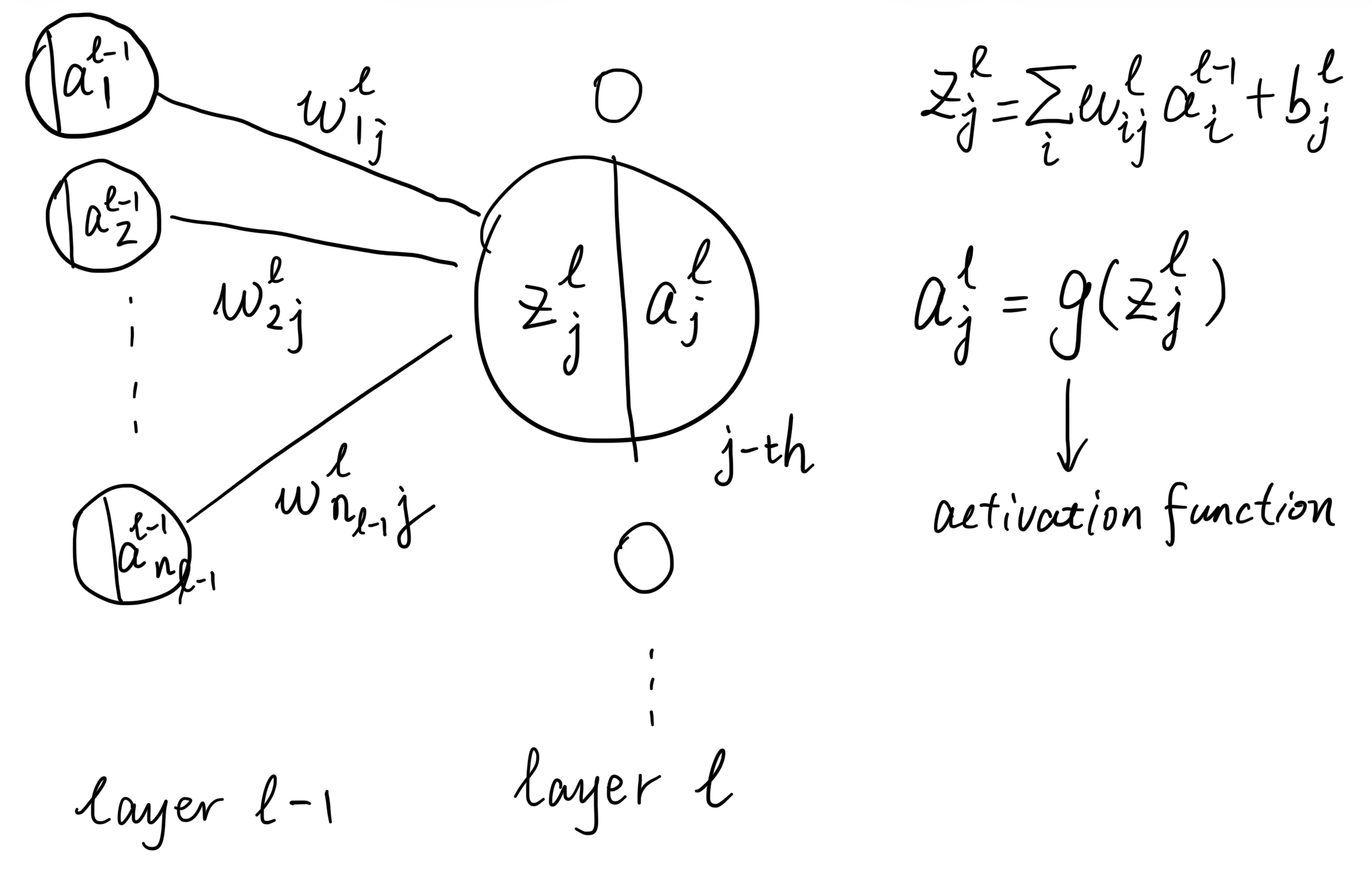
For the activation function $g(\cdot )$ on the $j$-th neuron in the layer $l$, the input:

• The weighted sum of inputs to the neuron: $z_j^l=\sum _i{w}_{ij}^l{a}_i^{l-1}+b_j^l$.

Output:

• The activated output of the neuron: $a_j^l=g(z_j^l)$

ImportantWhy applying the activation function to the neuron?

Activation functions introduce non-linearity into the model, allowing it to learn complex patterns in the data. Imagine if there were no activation functions in a neural network; it would essentially be a linear model.

Activation Functions

ImportantWhat activation functions are commonly used?

Common activation functions include:

ImportantWhy don’t we use binary step function as activation function?

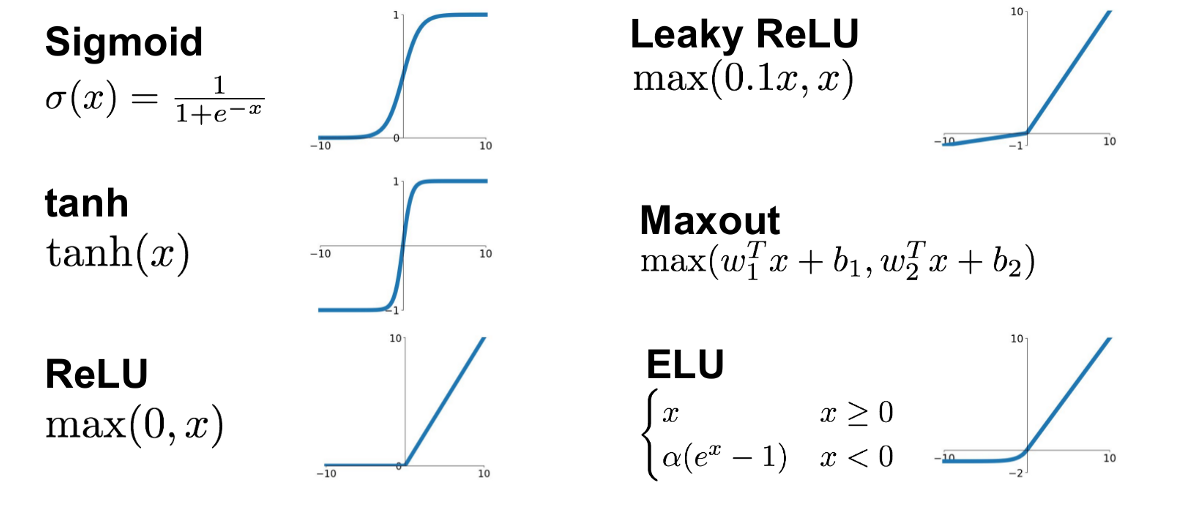
According to the literal meaning of “activation”, the binary step function seems to be a good choice, as it clearly defines whether a neuron is activated (output 1) or not (output 0). However, it cannot be differentiated at the step point, and its derivative is zero elsewhere. This makes it unsuitable for backpropagation, which relies on gradients to update the parameters during training.

Sigmoid

ImportantWhat is a Sigmoid function?

Sigmoid function is a mathematical function that maps any real-valued number into the range (0, 1). It has an “S”-shaped curve and is defined by the formula (Please note the English word “sigmoid” means “S-shaped”):

$$\text{Sigmoid}(x)=\frac{1}{1+e^{-x}}$$

Sigmoid function is the smooth version of the binary step function, making it differentiable for the backpropagation to work properly.

ImportantWhat are the pros and cons of Sigmoid activation function?

Pros:

• It maps input values to an output range between 0 and 1 (like a probability), making it suitable for binary classification tasks.
• Smooth gradients, which helps in optimization.
• Very much biologically plausible, as it mimics the firing rate of biological neurons.

Cons:

• Prone to vanishing gradient problem, which can hinder the training of deep networks.
• Outputs are not zero-centred. The zig-zag phenomenon can occur during optimization, which can lead to inefficient weight updates during training.
• Computationally expensive due to the exponential function.

ImportantWhat is the vanishing gradient problem?

The backpropagation computes the gradient of the loss function with respect to each layer’s parameters from the last layer backwards. The chain rule is applied, which means the gradients are multiplied by derivatives layer by layer. From the computation graph of neural network, we can see that the gradients are multiplied with the weights $w$, activation values $a$ and activation function derivative $g^{\prime }(z)$.

For some activation functions like Sigmoid and Tanh, their derivatives $g^{\prime }$ can be very easy to become small (close to 0) for certain input ranges:

• The derivative of the sigmoid function is ${\sigma }^{\prime }(x)=\sigma (x)(1-\sigma (x))$, which reaches its maximum value of $0.25$ at $x=0$. For most input values, the derivative is much smaller than $0.25$ (called saturated);
• The derivative of the tanh function is $1-{\tanh }^2(x)$, which approaches $0$ very quickly as $x$ moves away from $0$ in either direction.

When this small values multiply the gradients during backpropagation for multiple layers, the gradients can become very small, which stops the network from learning further. This is known as the vanishing gradient problem. The more layers there are, the more severe the problem can be; the closer to the input layer, the more serious the vanishing gradient becomes.

ImportantWhat is the zig-zag phenomenon?

From the computation graph of neural network, we can see that the path from the loss to a parameter (such as $w_{12}^{L-1}$ in the example) includes the $z$ to the parameter $\frac{\partial z_2^L}{\partial w_{12}^{L-1}}$ at last. This term is the activation value, in this example $a_1^{L-1}$. That is, the gradient of a parameter is proportional to the activation value of the neuron in the previous layer.

Suppose the activation function of the previous layer is Sigmoid, whose output is always positive. Then, for all parameters connecting to a neuron in the current layer (i.e., $w_{ij}^l$ with fixed $j$ and varying $i$), their gradients will have the same sign.

As a result, the parameters are divided into groups. For the parameters in the same group, they will always be updated in the same direction (either all increase or all decrease). This limits the freedom of parameter updates.

We illustrate a group in a 2D space below. Since the gradients have the same sign, the parameters will be updated either to the top-right or bottom-left. If the optimal solution happens to be the bottom-right direction (which is more likely in high-dimensional space), the zig-zag phenomenon occurs.

Zig-Zag.

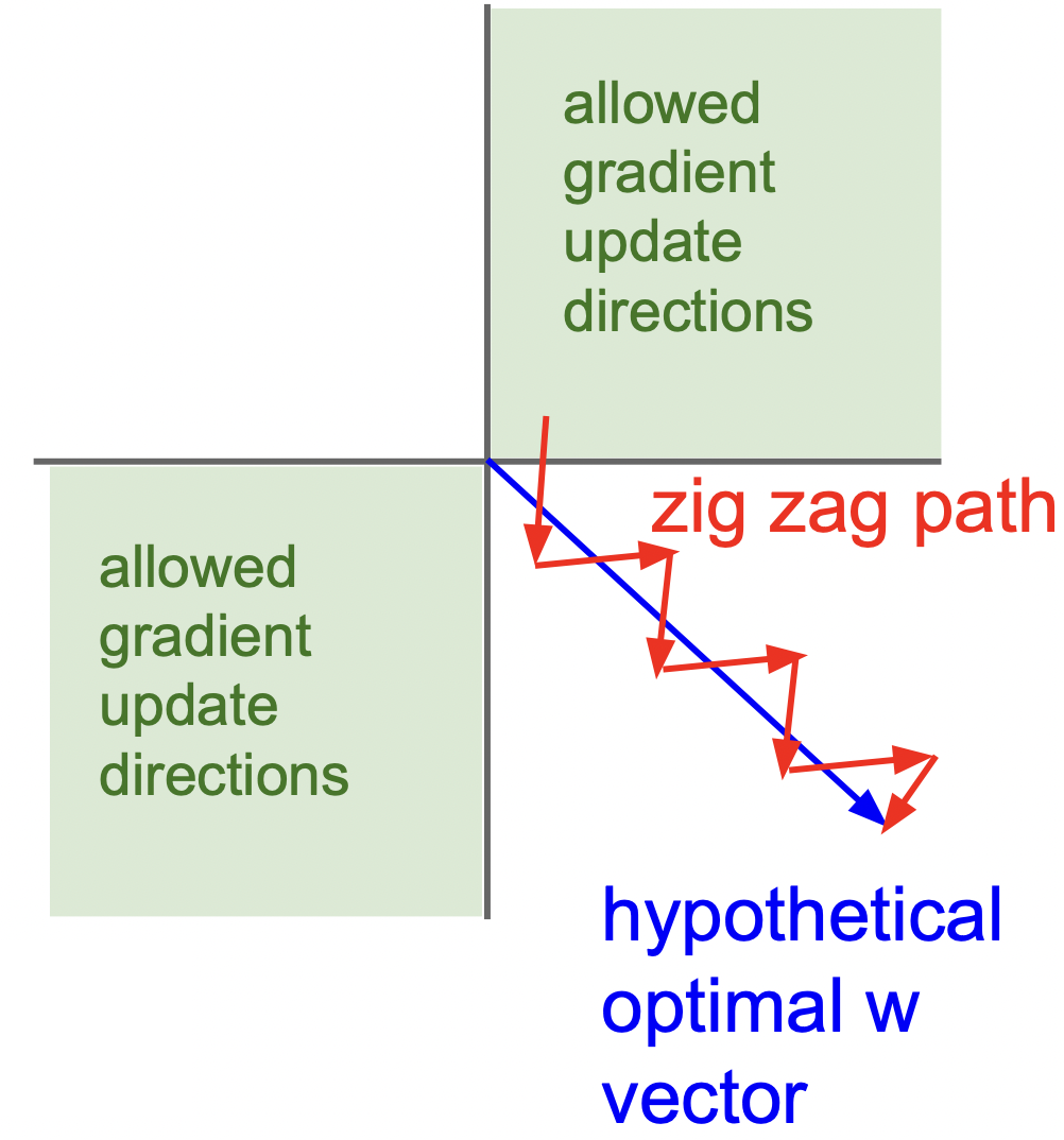
The optimal solution can be reached much faster if the parameters can be updated in the bottom-right direction. Therefore, zig-zag phenomenon can lead to inefficient parameter updates during training.

ImportantWhy is a zero-centred activation function preferred?

In the above zig-zag phenomenon, we see that the problem arises because the activation function’s output is always positive. If the activation function can produce both positive and negative outputs, the gradients of parameters connecting to a neuron in the current layer can have different signs. This allows for more flexible parameter updates.

The most ideal case is that the activation function can output both positive and negative values at the same odds. This would require the activation function to be zero-centred. Zero-centred activation function makes it more likely for the gradients of parameters in the same group to have different signs, thus reducing the zig-zag phenomenon and improving training efficiency.

TipWho used Sigmoid activation function?

Sigmoid is one of the earliest activation functions used in neural networks. It was widely used in 1980s’ perceptrons and multi-layer perceptrons (MLP). It was no longer popular after the 2010s due to its drawbacks.

Tanh

ImportantWhat is a Tanh function?

Tanh function is a mathematical function that maps any real-valued number into the range (-1, 1). It also has an “S”-shaped curve: $$\text{Tanh}(x)=\frac{e^x-e^{-x}}{e^x+e^{-x}}$$

Tanh is a scaled and shifted version of the Sigmoid function, making it zero-centred:

$$\text{Tanh}(x)=2\cdot \text{Sigmoid}(2x)-1$$

ImportantWhat are the pros and cons of Tanh activation function?

Tanh inherits most of the advantages and disadvantages of Sigmoid, except it is zero-centred, making zig-zag phenomenon less severe.

TipWho used Tanh activation function?

Tanh as improvement of Sigmoid was also widely used in 1980s’ perceptrons and multi-layer perceptrons (MLP). It is also used in some recurrent neural networks (RNNs) such as LSTM and GRU.

ReLU and Its Variants

ImportantWhat is a ReLU function?

ReLU (Rectified Linear Unit) is an activation function defined as: $$\text{ReLU}(x)=max(0,x)=\{\begin{array}{ll}x& x>0\\ 0& x\le 0\end{array}$$ It outputs the input directly if it is positive; otherwise, it outputs zero. The name was given by a paper in 2011: (Glorot, Bordes, and Bengio 2011).

ImportantHow does ReLU activation function work in forward and backward propagation?

The logic of ReLU and its derivative is simple: a neuron has two states—active or inactive.

• Active ($z_j^l>0$ so $a_j^l>0$): the forward value and backpropagated gradient pass through unchanged.
• Inactive ($z_j^l\le 0$ so $a_j^l\le 0$): both the forward value and gradient are blocked, becoming 0.

Formally: g(z_j^l) = $$\{\begin{array}{ll}{a}_j^l& a_j^l>0\\ 0& a_j^l\le 0\end{array}$$ , g’(a_j^l) = $$\{\begin{array}{ll}1& a_j^l>0\\ 0& a_j^l\le 0\end{array}$$

This highlights ReLU’s simplicity: it either lets information flow or blocks it completely.

ImportantReLU function seems to be indifferentiable at 0. Why does it still work in backpropagation?

Although the ReLU function is not differentiable at 0, it is still usable in backpropagation because we can define the gradient at that point. In practice, we often set the gradient to either 0 or 1 at $z_j^l=0$, and this choice does not significantly affect the overall training process. The key idea is that during backpropagation, we only need to know whether a neuron is active or inactive, which is determined by the sign of its input.

As for the binary step function, it is not differentiable at the step point, and its derivative is zero elsewhere. This makes all gradients zero basically, preventing any learning from occurring. That is the main problem.

ImportantWhat are the pros and cons of ReLU activation function?

Pros:

• No vanishing gradient problem in the positive part;
• Simple function, very efficient to compute.

Cons:

• Outputs are not zero-centred. The zig-zag phenomenon can occur during optimization, which can lead to inefficient weight updates during training.
• The “dying ReLU” problem: Neurons can be “dead” if the activation is negative, making the parameters connected to it not updated.

ImportantWhat happened when a ReLU neuron is “dead”? Why?

From the computation graph of neural network, we can see that the path from the loss to a parameter (such as $w_{12}^{L-1}$ in the example) includes the $z$ to the parameter $\frac{\partial z_2^L}{\partial w_{12}^{L-1}}$ at last. This term is the activation value, in this example $a_1^{L-1}$. That is, the gradient of a parameter is proportional to the activation value of the neuron in the previous layer.

ReLU function maps all negative inputs to zero. This means that the gradients of all parameters connected to this neuron will be multiplied by zero during backpropagation, resulting in zero gradients. The derivative of the ReLU activation function is also zero for negative inputs. This is multiplied in the chain rule as well, thus also results in zero gradients. Consequently, these parameters will not be updated during training.

Statistically, there is a 50% chance for a ReLU neuron to be “dead” (i.e., its input is negative) for any given input. It means that, on average, half of the parameters cannot be updated in each training step. This can affect the efficiency of training.

This is even a risk that some neurons may never be activated during the entire training process, leading to a portion of the network being undertrained or not trained at all.

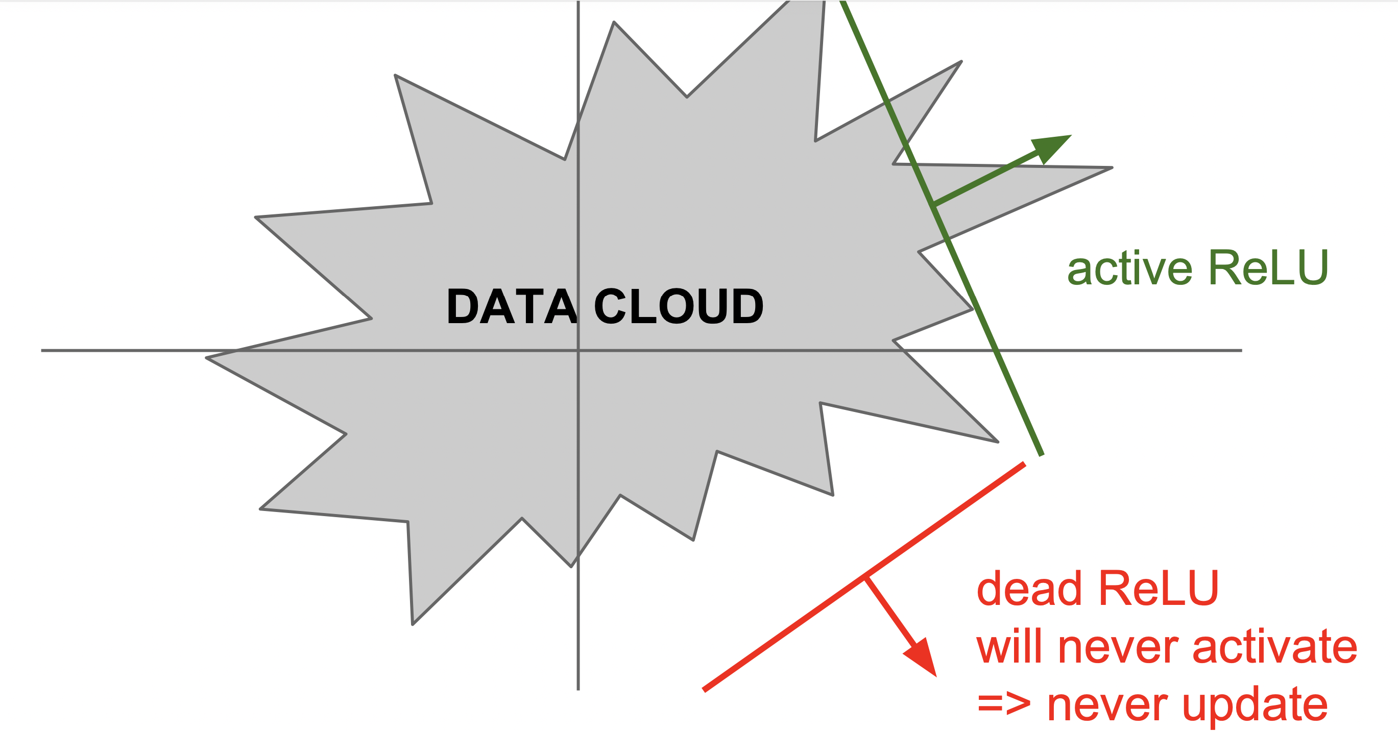
We assume a ReLU neuron receives two inputs from the previous layer, with weights $w_1$, $w_2$ and bias $b$. The neuron is activated if the weighted sum of inputs is greater than 0, i.e., $a_j^l=w_1{o}_1^{l-1}+w_2{o}_2^{l-1}>0$. The boundary condition for activation is $w_1{o}_1^{l-1}+w_2{o}_2^{l-1}=0$, which is a straight line in the 2D space of $(o_1^{l-1},o_2^{l-1})$. We illustrute this in the figure above. The training data passed in the layer forms a data cloud. A complete dead ReLU neuron happens when the data cloud is entirely on one side of the line. No training data can activate the neuron, so the parameters $w_1$, $w_2$, $b$ will never be updated, making the line fixed.

A bad and unstable optimizer (for example, an optimizer with a huge learning rate) may produce such weights and bias, making the neuron completely dead.

Please note, the data cloud in a layer is the representation of the original input data, not the original input data itself. Therefore, it is not fixed and can change during training, so there is still a chance for the neuron to be re-activated in the future. For further analysis, please refer to (Lu et al. 2019).

TipWho used ReLU activation function?

ReLU was first proposed to be used in neural networks by (Glorot, Bordes, and Bengio 2011). It is then used in the famous AlexNet convolutional neural network, significantly improving training speed and winning the ImageNet competition.

This led to the rapid popularization of ReLU in the deep learning community. Since then, almost all convolutional neural networks (CNNs) and most deep neural networks (DNNs) have adopted ReLU or its variants.

ImportantWhat are the ReLU function variants?

ReLU has several variants designed to address its drawbacks:

• Leaky ReLU: Allows a small, non-zero gradient when the unit is inactive (i.e., $z_j^l<0$):

$$\text{Leaky ReLU}(x)=max(0.1x,x)=\{\begin{array}{ll}x& x>0\\ \alpha x& x\le 0\end{array}$$

where $\alpha$ is a small constant (e.g., 0.01).

• Parametric ReLU (PReLU): Similar to Leaky ReLU, but the slope for negative inputs is learned during training.

• Exponential Linear Unit (ELU): Like ReLU, but it has a smooth exponential curve for negative inputs:

$$\text{ELU}(x)=\{\begin{array}{ll}x& x>0\\ \alpha (e^x-1)& x\le 0\end{array}$$

ImportantWhat are the pros and cons of ReLU activation function variants?

Leaky ReLU, PReLU, and ELU are designed to address the “dying ReLU” problem. There are small gradients for negative inputs, allowing the parameters to be updated even when the neuron is inactive.

The pros and cons of these variants are similar to ReLU, with the added benefit of mitigating the “dying ReLU” problem. In addition, ELU uses an exponential function for negative inputs, which can introduce additional computational overhead compared to ReLU and Leaky ReLU.

TipWho used ReLU activation function variants?

ReLU variants are proposed after ReLU became popular:

• Leaky ReLU was proposed by (Maas et al. 2013).
• PReLU was proposed by (He et al. 2015).
• ELU was proposed by (Clevert, Unterthiner, and Hochreiter 2015).

Most people still use ReLU due to its simplicity and efficiency. However, in some cases, especially when training very deep networks, these variants can provide better performance.

Maxout

ImportantWhat are the Maxout function?

Maxout is simply a function that takes the maximum value from multiple inputs:

$$\text{Maxout}(x_1,x_2,\dots ,x_k)=max(x_1,x_2,\dots ,x_k)$$

ImportantMaxout has multiple inputs. How can it work as an activation function?

Maxout can aggregate multiple neuron activations from the previous layer. It simply takes the maximum of multiple neuron activations. The number of inputs $k$ is a hyperparameter that can be tuned.

Maxout is sort of a generalization of ReLU. ReLU can be seen as a special case of Maxout with two inputs: the input itself and zero. Therefore, Maxout can be viewed as a more flexible activation function that can learn to select the most relevant features from multiple inputs.

ImportantWhat are the pros and cons of Maxout activation function?

Pros:

• Maxout can approximate any convex function, making it more flexible than ReLU or Sigmoid.
• Solves “dying ReLU” problem, since it doesn’t zero out all negative inputs, neurons don’t get stuck inactive.

Cons:

• More parameters: Each Maxout neuron equals $k$ linear units, increasing the number of parameters significantly.

TipWho used Maxout activation function?

Maxout was proposed in 2013 by (Goodfellow et al. 2013). It is rarely used in modern architectures, because ReLU and its variants (Leaky ReLU, GELU) are simpler and often perform just as well.

TipHow to choose an activation function?

The activation function forms the backbone of a neural network. The choice of activation function can significantly impact the performance of a neural network.

In general practice, ReLU and its variants (Leaky ReLU, GELU) are the most commonly used activation functions in modern neural networks due to their simplicity and effectiveness. Sigmoid and Tanh are less commonly used in hidden layers but may still be used in output layers for specific tasks (e.g., Sigmoid for binary classification). If there is no specific reason to choose another activation function, ReLU is usually a safe and effective choice.

References

Clevert, Djork-Arné, Thomas Unterthiner, and Sepp Hochreiter. 2015. “Fast and Accurate Deep Network Learning by Exponential Linear Units (Elus).” arXiv Preprint arXiv:1511.07289 4 (5): 11.

Glorot, Xavier, Antoine Bordes, and Yoshua Bengio. 2011. “Deep Sparse Rectifier Neural Networks.” In Proceedings of the Fourteenth International Conference on Artificial Intelligence and Statistics, 315–23. JMLR Workshop; Conference Proceedings.

Goodfellow, Ian, David Warde-Farley, Mehdi Mirza, Aaron Courville, and Yoshua Bengio. 2013. “Maxout Networks.” In International Conference on Machine Learning, 1319–27. PMLR.

He, Kaiming, Xiangyu Zhang, Shaoqing Ren, and Jian Sun. 2015. “Delving Deep into Rectifiers: Surpassing Human-Level Performance on Imagenet Classification.” In Proceedings of the IEEE International Conference on Computer Vision, 1026–34.

Lu, Lu, Yeonjong Shin, Yanhui Su, and George Em Karniadakis. 2019. “Dying Relu and Initialization: Theory and Numerical Examples.” arXiv Preprint arXiv:1903.06733.

Maas, Andrew L, Awni Y Hannun, Andrew Y Ng, et al. 2013. “Rectifier Nonlinearities Improve Neural Network Acoustic Models.” In Proc. Icml, 30:3. 1. Atlanta, GA.