Dynamic programming is an algorithm design paradigm for solving complex problems by breaking them down into simpler subproblems.
Suppose a algorithmic problem has a solution
This is a recursive structure, however, we don’t do recursion directly but in the dynamic programming way. Once the problem can be easily broken down into smaller subproblems, the way that dynamic programming solves the problem is to start from the base case (like
Problems with the above two properties can also be solved using both dynamic programming and divide-and-conquer. However, the key difference between dynamic programming and divide-and-conquer is that dynamic programming is used when the subproblems overlap, meaning that the same subproblems are solved multiple times. In contrast, divide-and-conquer is used when the subproblems are independent, meaning that each subproblem is solved only once.
Because the subproblems overlap, using recursion directly to solve the problem would result in a lot of redundant calculations, leading to an exponential time complexity. Dynamic programming avoids this by storing the solutions to the subproblems in a table (usually an array or a matrix) and reusing them when needed, resulting in a polynomial time complexity.
The Fibonacci sequence is a classic example of a problem that can be solved using dynamic programming. The transition function is explicitly defined in the problem. The Fibonacci sequence is defined as follows:
Let compute
The naive recursive approach to compute
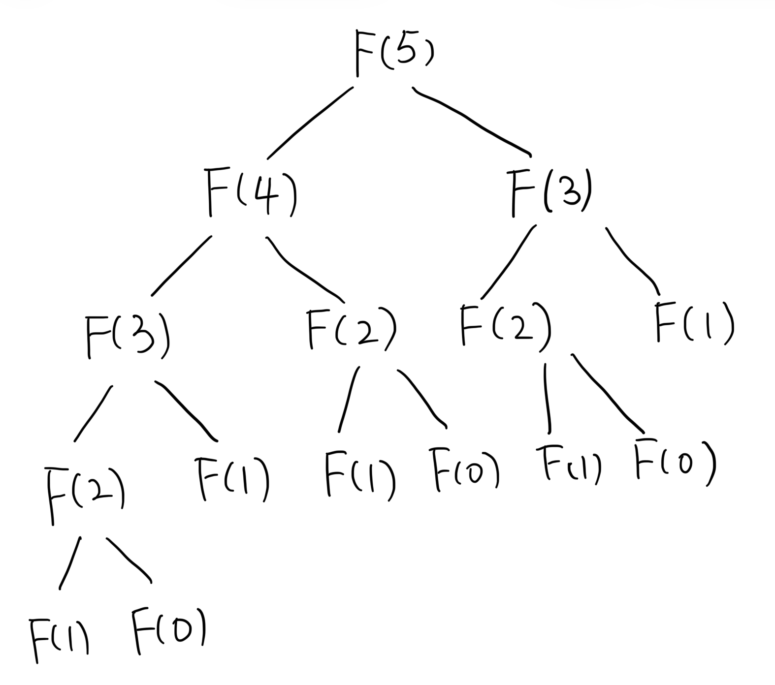
However, we can use dynamic programming to solve this problem efficiently by storing the results of the subproblems in an array and reusing them when needed. We can compute

If a problem has the following properties, we can use dynamic programming to solve it:
- The problem requires an answer that is a value, rather than a set of choices.
- The solution to the bigger problem can be constructed efficiently from solutions to smaller subproblems.
- The subproblems overlap, meaning that the same subproblems are solved multiple times.
Dynamic programmed variables can take various forms depending on the problem being solved.
- One DP variable:
- The variable usually has a multi-step formula, where the step sizes are determined by some conditions in the problem. Example: Fibonacci sequence, knapsack problem.
- Two DP variable:
- Two explicit separate things in the problem, which often corresponds to two DP variables.
- Two DP variables for one thing in the problem. These two variables likely represent some dual concepts, like left / right, min / max, etc.
- Two-dimensional DP variable:
- The problem involves a 2D thing, where the DP variable naturally becomes two-dimensional.
- Intervals: The problem involves intervals or ranges, where the DP variable is defined on the start and end points of the intervals.
- Tree/Graph-like DP variable:
- The problem involves a tree or graph structure, where the DP variable is defined on the nodes or edges of the tree/graph.
The dynamic programmed variable and its structure are usually not as simple as a one-dimensional array with one-step formula.
Optimal value (min / max / etc), ways to do something (number of ways, list of ways, etc), feasibility (whether something is possible or not), etc.
Some problems requires the argument that achieves the optimal value, which can be tracked using an auxiliary array during the DP process.