Backpropagation – Shawn’s Blog

My takeaway series follow a Q&A format to explain AI concepts at three levels:

Conceptual Level

Anyone with general knowledge can understand them.

Implementation Level

For anyone who wants to dive into the code implementation details of the concept.

Mathematical Level

For anyone who wants to understand the mathematics behind the technique.

What is backpropagation?

Backpropagation is the core procedure of the optimization algorithms for training neural networks. The optimization algorithm repeatedly updates the parameters of the network to minimize the difference between the predicted output and the actual target values. Backpropagation computes gradients for the optimization algorithm to use.

What is the input and output of backpropagation?

In each training step of a neural network, a forward and a backward pass are performed. The backward pass is the backpropagation process.

Input:

The loss \(l(f(\mathbf{x}; \theta), y)\) between the predicted output \(f(\mathbf{x}; \theta)\) and the target value \(y\), computed from the forward pass.
- The forward pass takes the input data \(\mathbf{x}\) and passes it through the network to produce the predicted output, as well as the loss.

Output:

The gradients of the loss with respect to parameters in the network \(\frac{\partial l(f(\mathbf{x}; \theta), y)}{\partial \theta}\).

What are the gradients?

In math, the gradient is a vector that contains all the partial derivatives of a multivariable function with respect to each variable. It points in the direction of the steepest increase of the function. This information is crucial for optimization algorithms to update the parameters effectively.

The loss function in neural network training is a multivariable function of the parameters \(\theta\) (weights \(w\)s and biases \(b\)s). \(\frac{\partial l(f(\mathbf{x}; \theta), y)}{\partial \theta}\) is a vector that contains all the partial derivatives of the loss with respect to each parameter in \(\theta\).

Strictly speaking, a gradient is a vector, not a single value. However, we often refer to the single partial derivative for each parameter, e.g., \(\frac{\partial l(f(\mathbf{x}; \theta), y)}{\partial w_{ij}^l}\), as the gradient for that parameter, as a vector can be one-dimensional. Moreover, we say “gradients” rather than “gradient” most of the time, as we can divide the parameters into groups such as by layer, and refer to the gradients of each group. (Note that the backpropagation also computes the gradients layer by layer, see below.)

What are the gradients computed by backpropagation used for?

The gradients are the core information used to update the parameters of the network by the optimization algorithm. The gradients computed by backpropagation are first-order gradients.

The first-order gradients can be used by first-order optimization algorithms like gradient descent, while the second-order gradients can be used by second-order optimization algorithms like Newton’s method. In deep learning, the optimization algorithms are usually simple first-order algorithms due to the high computational cost of second-order algorithms, that is gradient descent and its variants (e.g., SGD, Adam). Take gradient descent as an example, the parameters are updated as follows:

\[\theta \leftarrow \theta - \eta \frac{\partial l(f(\mathbf{x}; \theta), y)}{\partial \theta}\]

where \(\eta\) is the learning rate, controlling the step size of the update.

How does backpropagation compute the gradients?

Backpropagation computes the gradients of the loss, where the loss is a composite function of the parameters (composed by the loss function \(l\) and the neural network model \(f\), where \(f\) is a big multivariable composite function of the parameters). In calculus, the derivative of a composite function can be computed by the chain rule. Therefore, the backpropagation algorithm is just an application of the chain rule.

The chain rule for a multivariable composite function is as follows. It is basically summing the derivatives along all the paths from the dependent variable to the independent variable.

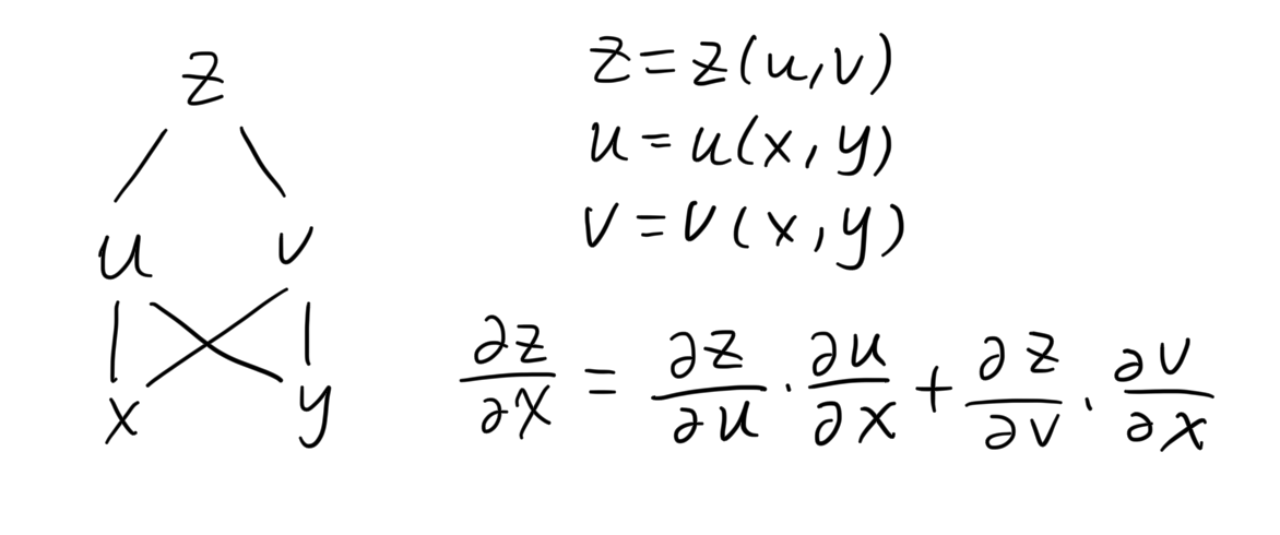
The composition relation between the variables in the function can be illustrated as above, which is called computation graph. For the loss function in neural network training (suppose a feed-forward network for regression problem), the computation graph is as follows:

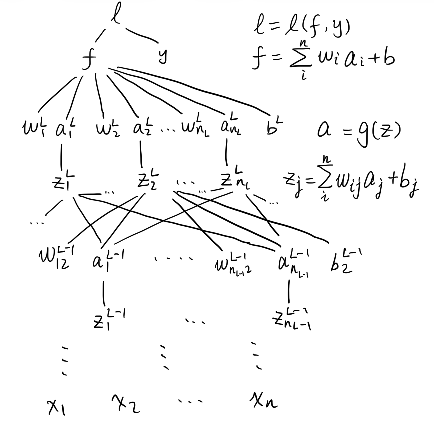
Figure 1: Chain rule in neural network. Please note this looks similar but not entirely the same as the neural network illustration.

All \(w\)s and \(b\)s belong to the model parameters \(\theta\), so the target gradient to compute are \(\frac{\partial l}{\partial w}\) and \(\frac{\partial l}{\partial b}\). To compute them, taking \(\frac{\partial l}{\partial w_{12}^{l-1}}\) as an example, there is one path only for \(l\) to \(w_{12}^{l-1}\):

\[\begin{align} l &= l(f,y) =\frac12 (f-y)^2\\ f &= \sum_i^{n_L}w^{l}_ia^{l}_i+b^{l} \\ a^{l}_2 &= g(z^{l}_2) \\ z^{l}_2 &= \sum_i^{n_{L-1}}w^{l-1}_{i2} a^{l-1}_i + b_2^{l-1} \\ \end{align}\]

According to chain rule,

\[\begin{align} \frac{\partial l}{\partial w_{12}^{l-1}} &= \frac{\partial l}{\partial f} \cdot \frac{\partial f}{\partial a^{l}_2} \cdot \frac{\partial a^{l}_2}{\partial z^{l}_2} \cdot \frac{\partial z^{l}_2}{\partial w_{12}^{l-1}}\\ &= 2(f-y) \cdot w^{l}_2 \cdot g'(z^{l}_2) \cdot a^{l-1}_1\\ \end{align}\]

Why is it called backpropagation?

We can see from the above example that the most efficient way to compute all the gradients is to start from the loss and compute the gradients layer by layer backwards. The gradient of a layer is computed based on the gradient of the next layer, seemingly propagating back through the network. This is why it is called backpropagation.