My takeaway series follow a Q&A format to explain AI concepts at three levels:
Anyone with general knowledge can understand them.
For anyone who wants to dive into the code implementation details of the concept.
For anyone who wants to understand the mathematics behind the technique.
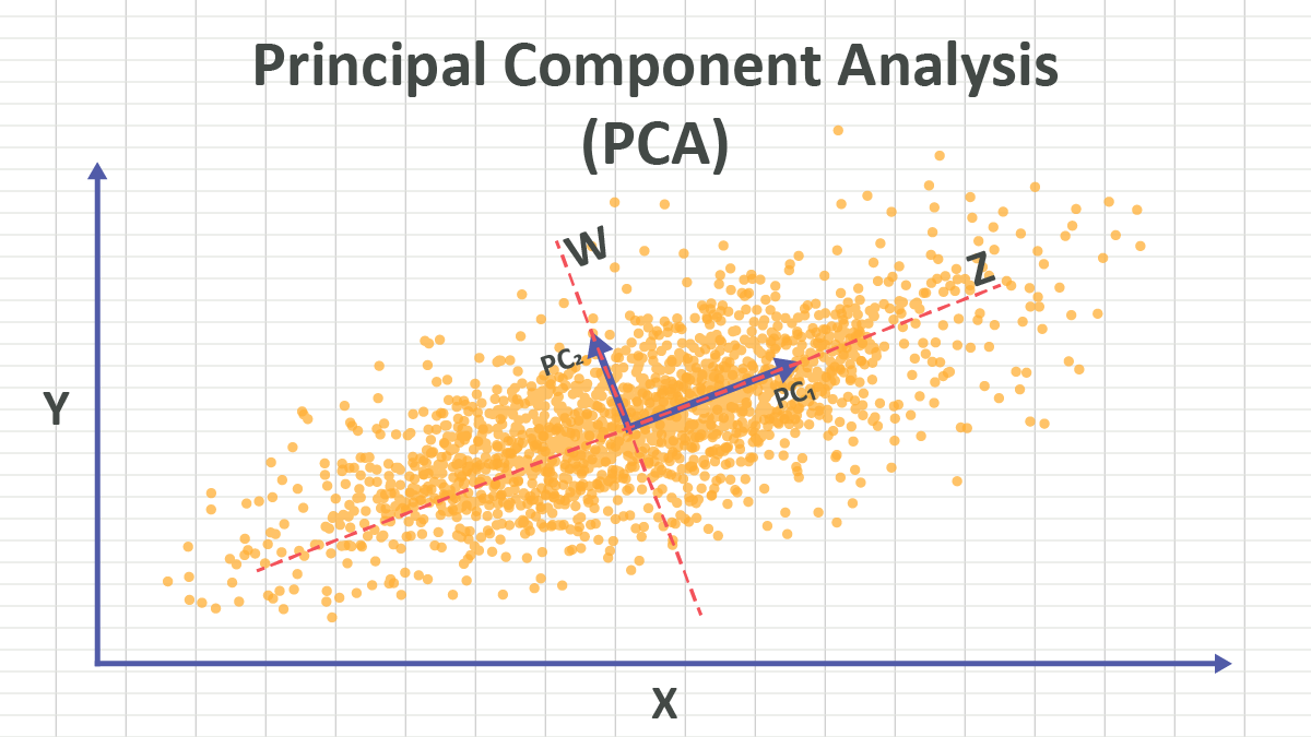
Principal Component Analysis (PCA) is a dimensionality reduction technique. It finds the principal components in high-dimensional data and projects the data onto a lower-dimensional space. In AI context, PCA is an unsupervised learning algorithm.
PCA is a data dimensionality reduction technique.
Inputs:
- A dataset with \(n\) samples and \(d\) features, represented as a matrix \(\mathbf{X} \in \mathbb{R}^{n \times d}\), where each row corresponds to a sample and each column corresponds to a feature with \(d\) dimension.
Outputs:
- A transformed dataset with \(n\) samples and \(k\) principal components, represented as a matrix \(\mathbf{Z} \in \mathbb{R}^{n \times k}\), where \(k < d\).
PCA is done by SVD (Singular Value Decomposition). The steps are as follows:
- Standardize the data: Subtract the mean and divide by the standard deviation for each feature to ensure that each feature contributes equally to the analysis.
\[\mathbf{X} = \frac{\mathbf{X} - \mu}{\sigma}\]
- Perform SVD on the standardized data matrix:
\[\mathbf{X} = \mathbf{U} \boldsymbol{\Sigma} \mathbf{V}^T\]
where \(\mathbf{U} \in \mathbb{R}^{n \times n}\) is the left singular vectors, \(\boldsymbol{\Sigma} \in \mathbb{R}^{n \times d}\) is a diagonal matrix with singular values, and \(\mathbf{V}^T \in \mathbb{R}^{d \times d}\) is the right singular vectors.
- Choose the top \(k\) columns of \(\mathbf{U}\) corresponding to the largest singular values in \(\boldsymbol{\Sigma}\):
\[\mathbf{U}_k = (\mathbf{u}_1, \cdots, \mathbf{u}_k)\]
- Transform the data: Project the original standardized data onto the new feature space using the chosen principal components.
\[\mathbf{z}_1 = \mathbf{X} \cdot \mathbf{u}_1 \in \mathbb{R}^{n}\] \[\mathbf{z}_2 = \mathbf{X} \cdot \mathbf{u}_2 \in \mathbb{R}^{n}\] \[\cdots\] \[\mathbf{z}_k = \mathbf{X} \cdot \mathbf{u}_k \in \mathbb{R}^{n}\]
Each principal component \(z_i\) represents a new feature that is a linear combination of the original features. This can be written in matrix form as:
\[\mathbf{Z} = \mathbf{X} \cdot \mathbf{U}_k \in \mathbb{R}^{n \times k}\]
- The feature projected onto the first principal component \(\mathbf{u}_1\) has the largest variance, the feature projected onto the second principal component \(\mathbf{u}_2\) has the second largest variance, and so on.
- The transformed feature are statistically uncorrelated to each other, that is, when a feature increases or decreases, the other features do not change in a predictable way.
These two properties make the new features:
- More informative and less redundant, because the features carrying more information (less variance) are preserved first, and less informative (more variance) features are discarded.
- More independent, because the features are uncorrelated.
\(\mathbf{U}_k\) is a linear transformation. In linear algebra we learned, a linear transformation is a mathematical operation that can substitute the original coordinate system with a new coordinate system. If there is no bias term, the new coordinate system is also based on the same origin point. In (PCA-visualization?), it looks like the new coordinate system moves away from the original coordinate system, that is because we have zero centred the data.
In PCA, the new coordinate system is defined by the principal components \(\mathbf{u}_i\). Since \(\mathbf{U}\) is an orthogonal matrix, the principal components \(\mathbf{u}_i\) are orthogonal to each other, so the new coordinate system is orthogonal.
Standardizing the data is crucial before applying PCA because PCA is sensitive to the scale of the features. If the features are on different scales, PCA may give more importance to features with larger scales, leading to biased results. Standardization ensures that each feature contributes equally to the analysis by transforming them to have zero mean and unit variance.
SVD is a mathematical technique that decomposes a matrix into three other matrices. For a given matrix \(A \in \mathbb{R}^{m \times n}\), SVD decomposes it as follows:
\[A = U \Sigma V^T\]
where:
- \(U \in \mathbb{R}^{m \times m}\) is an orthogonal matrix whose columns are the left singular vectors of \(A\).
- \(\Sigma \in \mathbb{R}^{m \times n}\) is a diagonal matrix whose diagonal entries are the singular values of \(A\).
- \(V^T \in \mathbb{R}^{n \times n}\) is an orthogonal matrix whose columns are the right singular vectors of \(A\).
The singular values in \(\Sigma\) are non-negative and are typically arranged in descending order. The number of non-zero singular values is equal to the rank of the matrix \(A\).
To compute the SVD of a matrix \(A\), follow these steps:
- Compute the covariance matrix of \(A\):
\[C = A^T A\]
- Compute the eigenvalues and eigenvectors of the covariance matrix \(C\):
\[C v_i = \lambda_i v_i\]
Form the matrix \(V\) using the normalized eigenvectors \(v_i\) as columns.
Compute the singular values \(\sigma_i\) as the square roots of the eigenvalues:
\[\sigma_i = \sqrt{\lambda_i}\]
Form the diagonal matrix \(\Sigma\) using the singular values \(\sigma_i\).
Compute the left singular vectors \(U\) using the relationship:
\[U = A V \Sigma^{-1}\]
- The SVD of \(A\) is then given by:
\[A = U \Sigma V^T\]