graph TD
definition(What is Convolutional Neural Networks?) --> input-output(What are the inputs and outputs of CNN?)
definition --> architecture(What is the architecture of a typical CNN?)
architecture --> input-output-conv-layer(What is the input and output of convolutional layer?)
input-output-conv-layer --> feature-map(Why is it called feature map?)
input-output-conv-layer --> convolutional-layer(What does the convolutional layer do?)
convolutional-layer --> convolution-name(What is it called "convolution"?)
convolutional-layer --> kernel-slide(In which way does the kernel slide over the input feature map exactly?)
convolutional-layer --> convolution-operation(What is the convolution operation trying to achieve?)
kernel-slide --> why-padding(Why do we need padding?)
kernel-slide --> common-padding-values(What are the common values for padding?)
kernel-slide --> output-size-conv-layer(What is the output size of a convolutional layer?)
convolutional-layer --> conv-down-sampling(Is the convolutional layer a down-sampling operation?)
convolutional-layer --> conv-vs-fc(What is the difference between convolutional layer and fully connected layer?)
convolutional-layer --> why-conv-better(Why is the convolutional layer better at dealing with image data?)
kernel-slide --> num-params-conv(How many parameters are there in a convolutional layer?)
num-params-conv --> input-image-size-affect(Does the input image size affect the size of the CNN?)
architecture --> input-output-pooling-layer(What is the input and output of pooling layer?)
input-output-pooling-layer --> pooling-layer(What does the pooling layer do?)
pooling-layer --> types-of-pooling(What are the types of pooling operation?)
pooling-layer --> pooling-down-sampling(What is the pooling layer a down-sampling operation?)
pooling-layer --> output-size-pooling-layer(What is the output size of a pooling layer?)
pooling-layer --> why-pooling(Why do we need pooling layers?)
architecture --> common-settings(What are the common settings of convolutional and pooling layers?)
architecture --> popular-cnn-architectures(What are the popular CNN architectures?)

click definition "#definition"
click input-output "#input-output"
click architecture "#architecture"
click input-output-conv-layer "#input-output-conv-layer"
click feature-map "#feature-map"
click convolutional-layer "#convolutional-layer"
click convolution-name "#convolution-name"
click kernel-slide "#kernel-slide"
click convolution-operation "#convolution-operation"
click why-padding "#why-padding"
click common-padding-values "#common-padding-values"
click output-size-conv-layer "#output-size-conv-layer"
click conv-down-sampling "#conv-down-sampling"
click conv-vs-fc "#conv-vs-fc"
click why-conv-better "#why-conv-better"
click num-params-conv "#num-params-conv"
click input-image-size-affect "#input-output-pooling-layer"
click input-output-pooling-layer "#input-output-pooling-layer"
click pooling-layer "#pooling-layer"
click types-of-pooling "#types-of-pooling"
click pooling-down-sampling "#pooling-down-sampling"
click output-size-pooling-layer "#output-size-pooling-layer"
click why-pooling "#why-pooling"
click common-settings "#common-settings"
click popular-cnn-architectures "#popular-cnn-architectures"
My takeaway series follow a Q&A format to explain AI concepts at three levels:
TipConceptual Level
Anyone with general knowledge can understand them.
WarningImplementation Level
For anyone who wants to dive into the code implementation details of the concept.
ImportantMathematical Level
For anyone who wants to understand the mathematics behind the technique.
These notes are taken when I was taking CV courses in my first year PhD. I’ve reorganised them into QA format.
TipWhat is Convolutional Neural Networks (CNN)?
Convolutional Neural Network (CNN) is a type of neural network designed for processing structured grid data, such as images. They are particularly effective for image recognition and classification tasks due to their ability to automatically learn spatial hierarchies of features from input images.
ImportantWhat are the inputs and outputs of CNN?
The CNN processes grid-like data, we take images as an example.
Inputs:
- An image \(\mathbf{x}\) represented as a 3D tensor of shape (height, width, channels), where height and width are the dimensions of the image, and channels represent the color channels (e.g., RGB).
Outputs:
- An output vector \(\mathbf{y}\) representing the class probabilities for classification tasks, or a feature map for other tasks.
ImportantWhat is the architecture of a typical CNN?

CNN does not refer to a specific architecture, but a class of neural networks. A typical CNN architecture is a sequence of
- Convolutional Layers: These layers apply convolution operations to the input data using learnable filters (kernels) to extract local features. Convolutional layers are parameterised layers.
- Pooling Layers: These layers perform down-sampling operations to reduce dimensions. Pooling layers are non-parameterised layers.
- Fully-Connected Layers: Same as layers in MLP.
The following types of layers are also sometimes used in CNN architectures:
- Deconvolutional Layers (Transposed Convolutional Layers): These layers perform the reverse operation of convolution, used for upsampling. Deconvolutional layers are parameterised layers.
- Up-pooling Layers: These layers perform up-sampling operations to increase dimensions. Up-pooling layers are non-parameterised layers.
ImportantWhat is the input and output of convolutional layer?
Input:
- A feature map that is a 3D tensor \(\mathbf{x}\) of shape \((H, W, C)\). It can be the input image or the output feature map from the previous layer.
Output:
- A feature map \(\mathbf{Y}\) of shape \((H', W', C')\).
TipWhy is it called feature map?
Feature map refers to the 3D tensor received and output by convolutional layers. An image is also a 3D tensor, where each channel is 2D and can be described as map. The image itself is a feature, so the whole thing can be feature map.
The input and output of convolutional layers do not necessarily have 3 channels, so they are not images. That’s why the term feature map is used.
ImportantWhat does the convolutional layer do?
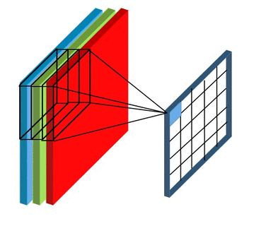
The convolutional layer has a set of smaller-sized kernels \((F_1, F_2, C)\), each of which is convolved with the input feature map to produce a 2D map. The activation maps from all kernels are stacked together to form the output feature map.
The convolution operation of one kernel to produce one 2D map is illustrated in (convolution-operation?). A kernel is a small 3D tensor with the same number of channels \(C\) as the input feature map. The kernel slides over the input feature map, performing element-wise multiplication and summation at each position to produce a single value in the output map. This process is repeated for all positions in the input feature map.
TipWhat is it called “convolution”?
The term “convolution” originates from the mathematical operation of convolution, which involves flipping one function and sliding it over another function to compute an dot product that expresses how the shape of one is modified by the other. In the context of CNNs, the kernel is not flipped, but the operation still involves sliding a smaller matrix (the kernel) over a larger matrix (the input feature map) and performing element-wise multiplication and summation, which is a dot product.
ImportantIn which way does the kernel slide over the input feature map exactly?
The output of the convolutional layer is a 3D tensor, so the kernel must slide uniformly over the input feature map. That is, the way the kernel slides over the input feature map and the kernel size are the same in between all channels.
The way that a kernel slides over the input feature map is determined by two hyperparameters:
- Stride: The number of pixels the kernel moves each time it slides over the input feature map. It can be specified separately for the horizontal and vertical directions.
- Padding: The number of pixels added to the border of the input feature map. It can also be specified separately for the horizontal and vertical directions.
TipWhat is the convolution operation trying to achieve?
The kernel slides over the input feature map to capture local features. The kernel size controls the receptive field of the local features. Different kernels can learn to detect different features, such as edges, textures, or patterns.
TipWhy do we need padding?
Padding can make sure the kernel can cover the corners of the input feature map. Without padding, the kernel cannot fully cover the corners, leading to loss of information at the edges of the input feature map.
TipWhat are the common values for padding?
The values for padding are:
- Zeros (called zero-padding);
- Replication of the nearest pixel values.
ImportantWhat is the output size of a convolutional layer?
Suppose:
- Input feature map size: \(W \times H \times C\);
- Number of kernels: \(K\);
- Kernel size: \(F_1 \times F_2\);
- Stride: \((S_1, S_2)\);
- Padding: \((p_1, p_2)\).
First, we can determine the output feature map depth \[C'\], which is equal to the number of kernels \[K\], because each kernel produces one 2D feature map, and all 2D feature maps are stacked together to form the output feature map.
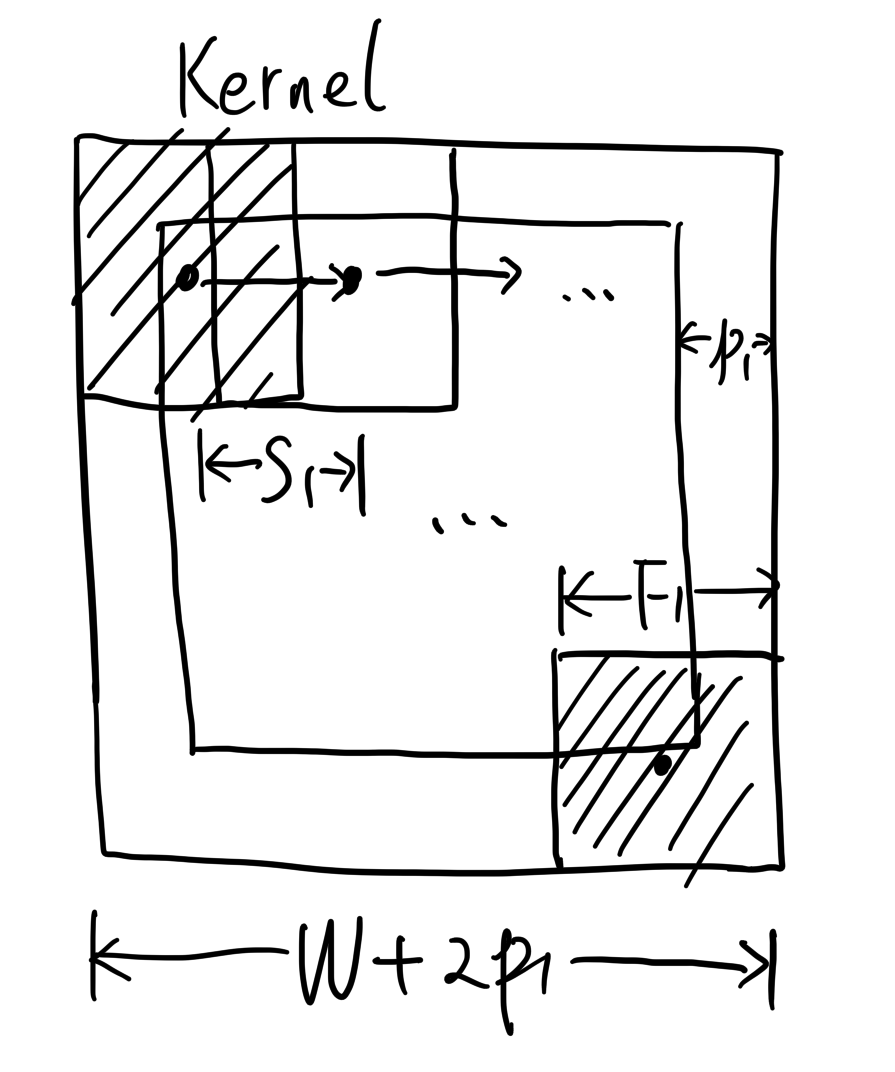
Then, we determine the output feature map width \[W'\] and height \[H'\]. Taking the horizontal direction as an example, after adding padding on both sides, the actual effective width of the image becomes \(W+2p_1\). The range that the kernel can slide over is \(W+2p_1 - 2 F_1\), and it can slide \((W+2p_1-F_1)/S_1\) times. Don’t forget the +1 at the end, since the kernel centre can be at both ends. This gives:
\[ W' = \frac{W+2p_1-F_1}{S_1} + 1 \]
Similarly, we have:
\[ H' = \frac{H+2p_2-F_2}{S_2} + 1 \]
Please note that the division in the formulas may not be exact. In such cases, add more padding to make it exact.
ImportantIs the convolutional layer a down-sampling operation?
When \(W'(H')<W(H)\), the convolutional layer is a down-sampling operation. As we see from the formula of \(W'\) and \(H'\), whether \(W'(H')<W(H)\) depends on the hyperparameters of the convolutional layer.
When the stride \(S_1(S_2)\) is greater than 1, the convolutional layer is a down-sampling operation. When the stride \(S_1(S_2)\) equals 1, whether it is a down-sampling operation depends on the kernel size \(F_1(F_2)\) and padding \(p_1(p_2)\). A larger kernel size and smaller padding are more likely to result in down-sampling. As padding goes meaningless when it is greater than kernel size, there is no choice that the convolutional layer is an up-sampling operation.
ImportantWhat is the difference between convolutional layer and fully connected layer?
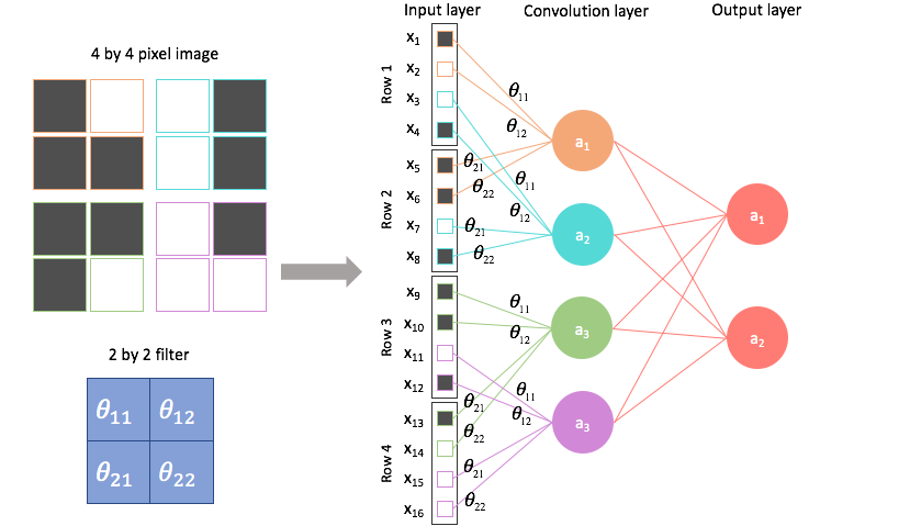
If we flatten the input and output feature maps into 1D vectors, we can see that the convolutional layer is similar to a fully connected layer: each input neuron is connected to each output neuron through weights, and each output neuron has an activation function.
However, these connections own two key features that are different from a fully connection:
- Local connectivity: Not all neurons are connected with weights; the weight matrix \[\mathbf{W}\] is sparse.
- Weight sharing: Many elements of \[\mathbf{W}\] share the same values, as they come from the same convolution kernel. They can be regarded as the same variable repeatedly applied in the composite function, having identical values and gradients.
These two features largely reduce the number of parameters in the convolutional layer compared to a fully connected layer.
TipWhy is the convolutional layer better at dealing with image data?
- Preserving spatial information: Compared with fully connected layers that flatten the input, the connection pattern of convolutional layers retains the notion of spatial position in an image, making them more suitable for image processing.
- Adaptation to scale variations: By using convolution kernels of different sizes (note: not within the same convolutional layer), both large-scale structures and fine details can be effectively captured.
ImportantHow many parameters are there in a convolutional layer, compared to a fully connected layer?
The weights are shared among all spatial locations in the input feature map, and all spatial locations use the same set of weights for convolution. Therefore, one kernel corresponds to one set of weights with a size of \(F_1\times F_2 \times C\). The total number of weights is \(F_1\times F_2 \times C \times K\), where \(K\) is the number of kernels.
If this is a fully connected layer, the number of input neurons is \(W \times H \times C\), and the number of output neurons is \(W' \times H' \times C'\). Therefore, the weight matrix size would be \(W \times H \times C \times W' \times H' \times C'\).
We can see that the number of parameters in a convolutional layer is significantly smaller than that in a fully connected layer, especially when the input feature map size \(W \times H\) is large.
ImportantDoes the input image size affect the size of the CNN?
No, because the convolutional layer is a local operation, and the weights are shared across all spatial locations. The number of parameters in a convolutional layer depends on the kernel size, number of kernels, and number of input channels, but not on the input image size.
TipWhat is the input and output of pooling layer?
The pooling layer also takes a feature map as input and produces a feature map as output.
Input:
- A feature map that is a 3D tensor \(\mathbf{x}\) of shape \((H, W, C)\). It can be the input image or the output feature map from the previous layer.
Output:
- A feature map \(\mathbf{Y}\) of shape \((H', W', C)\), which has the same number of channels as the input feature map.
ImportantWhat does the pooling layer do?
The pooling layer aggregates the pixels in a local neighbourhood to produce a single pixel in the output feature map. This applies to all channels independently. It doesn’t aggregate information across channels. The pooling layer is a non-parameterised layer, as the aggregation operation does not involve parameters.
The range of the local neighbourhood is determined by the filter size \((F_1, F_2)\) and stride \((S_1, S_2)\), similar to the convolutional layer.
ImportantWhat are the types of pooling operation?
The pooling operation can be:
- Max Pooling: Takes the maximum value in the local neighbourhood.
- Average Pooling: Takes the average value in the local neighbourhood.
ImportantWhat is the pooling layer a down-sampling operation?
Like the convolutional layer, whether the pooling layer is a down-sampling operation depends on its hyperparameters, but can never be an up-sampling operation.
The pooling layer is designed to use a down-sampling operation to reduce the spatial dimensions of the feature map. That’s why it doesn’t have padding as a hyperparameter, and the stride is usually set equal to the filter size to avoid overlapping regions.
ImportantWhat is the output size of a pooling layer?
Suppose:
- Input feature map size: \(W \times H \times C\);
- Filter size: \(F_1 \times F_2\);
- Stride: \((S_1, S_2)\);
The computation of the output feature map size \(W' \times H' \times C'\) is similar to that of the convolutional layer. The depth \(C'\) remains unchanged because pooling is performed independently on each channel. The width \(W'\) and height \(H'\) are computed as follows:
\[ W' = \frac{W-F_1}{S_1} + 1 \]
\[ H' = \frac{H-F_2}{S_2} + 1 \]
TipWhy do we need pooling layers?
Pooling layers are essential in CNNs for several reasons:
- Dimensionality Reduction: Pooling layers reduce the spatial dimensions of the feature maps, which decreases the number of parameters and computations in the network, leading to faster training and inference times.
- Avoiding Overfitting: By reducing the number of parameters, pooling layers help to mitigate overfitting, especially in deep networks.
TipWhat are the common settings of convolutional and pooling layers?
Convolution kernels are usually applied without distinguishing between horizontal and vertical directions, that is, \[F_1 = F_2, S_1 = S_2, p_1 = p_2\]
In addition, padding is typically chosen so that the convolution kernel exactly covers the image corners, determined by the kernel size:
\[p = \text{floor}(F/2)\]
Common hyperparameter settings include:
- \(3 \times 3\) kernel, stride 1, padding 1;
- \(5 \times 5\) kernel, stride 1 or 2, padding 2;
- \(1 \times 1\) kernel, stride 1, padding 0.
A \(1 \times 1\) kernel only fuses information along the depth (channel) dimension of each pixel, but it is still useful.
For pooling layers, filters are usually applied without padding, and the stride tends to equal the filter size (i.e., non-overlapping sampling). Similar to convolution kernels, they are typically square: \[F_1 = F_2\]
Common hyperparameter settings include:
- \(2 \times 2\) filter, stride 2, padding 0;
- \(3 \times 3\) filter, stride 2, padding 0.
TipWhat are the popular CNN architectures?
Some popular CNN architectures include:
- LeNet-5 (1998): One of the earliest CNN architectures, designed for handwritten digit recognition.
- AlexNet (2012): Won the ImageNet Large Scale Visual Recognition Challenge (ILSVRC) in 2012, significantly outperforming previous methods.
- VGGNet (2014): Known for its simplicity and depth, using very small (3x3) convolutional filters.
- GoogLeNet (Inception) (2014): Introduced the Inception module, which allows for more efficient computation by using multiple filter sizes in parallel.
- ResNet (2015): Introduced residual connections to allow for very deep networks, winning the ILSVRC 2015.
- U-Net (2015): Designed for biomedical image segmentation, featuring a U-shaped architecture with skip connections.
- DenseNet (2016): Each layer is connected to every other layer in a feed-forward fashion, improving information flow and gradient propagation.
- EfficientNet (2019): Uses a compound scaling method to scale up CNNs in a more structured way, achieving better performance with fewer parameters.